- Let's talk about Neural Networks.
- Some Basic Concepts Related to Neural Networks
- Weight and Bias initialization
- Activation Functions
- Why are deep neural networks hard to train?
- How to avoid Overfitting of Neural Networks?
- Step by Step Working of the Artificial Neural Network

Supervised learning can be used on both structured and unstructered data. For example of a structured data let's take house prices prediction data, let's also assume the given data tells us the size and the number of bedrooms. This is what is called a well structured data, where each features, such as the size of the house, the number of bedrooms, etc has a very well defined meaning.
In contrast, unstructured data refers to things like audio, raw audio, or images where you might want to recognize what's in the image or text (like object detection and OCR Optical character recognition). Here, the features might be the pixel values in an image or the individual words in a piece of text. It's not really clear what each pixel of the image represents and therefore this falls under the unstructured data.
Simple machine learning algorithms work well with structured data. But when it comes to unstructured data, their performance tends to take a quite dip. This where Neural Netowrks does their magic , which have proven to be so effective and useful. They perform exceptionally well on structured data.

As the Amount of data icreases, the performance of data learning algorithms, like SVM and logistic regression, does not improve infacts it tends to plateau after a certain point. In the case of neural networks as the amount of data increases the performance of the model increases.


Input layers:- Also known as Input Nodes are the input information from the dataset the features $x_1$ , $x_2$ , ..... $x_n$ that is provided to the model to learn and derive conclusions from. Input nodes pass the information to the next layer i.e Hidden layers.
Hidden layers:- It is the set of neurons where all the computations are performed on the input data. There can be any number of hidden layers in a neural network. The simplest network consists of a single hidden layer.
This is the layer where complex computations happen. The more your model has hidden layers, the more complex the model will be. This is kind of like a black box of the neural network where the model learns complex relations present in the data.
It is the process of updating and finding the optimal values of weights or ceofficients which helps the model to minimize the error (loss function). The weights are updated with the help of optimizers we talked about in Gradient Descent article. The weights of the network connections are repeatedly adjusted to minimize the difference between tha actual and the observed values. It aims to minimize the cost function by adjusting the network weights and biases. The cost funciton gradient determine the level of adjustment with respect to parameters like activation funciton , weights, biases etc.

After propagating the input features forward to the output layer through the various hidden layers consisting of different/same activation functions, we come up with a predicted probability of a sample belonging to the positive class ( generally, for classification tasks).Now, the backpropagation algorithm propagates backward from the output layer to the input layer calculating the error gradients on the way.Once the computation for gradients of the cost function w.r.t each parameter (weights and biases) in the neural network is done, the algorithm takes a gradient descent step towards the minimum to update the value of each parameter in the network using these gradients.


Output Layer:- From the diagram given above ther is only on node in the ouput layer, but don't think that is always like that in every neural network model. The number of nodes in the output layer completely depends upon the problem that we have taken. If we have a binary classification problem then the output node is going to be 1 but in the case of multi-class classification, the output nodes can be more than 1.

Its main objective is to prevent layer activation outputs from exploding or vanishing gradients during the forward propagation. If either of the problems occurs, loss gradients will either be too large or too small, and the network will take more time to converge if it is even able to do so at all.
If we initialized the weights correctly, then our objective i.e, optimization of loss function will be achieved in the least time otherwise converging to a minimum using gradient descent will be impossible.
Building even a simple neural network can be a confusing task and upon that tuning it to get a better result is extremely tedious. But, the first step that comes in consideration while building a neural network is the initialization of parameters, if done correctly then optimization will be achieved in the least time otherwise converging to a minima using gradient descent will be impossible.
Basic notations Consider an L layer neural network, which has L-1 hidden layers and 1 input and output layer each. The parameters (weights and biases) for layer l are represented as

The nodes in neural networks are composed of parameters referred to as weights used to calculate a weighted sum of the inputs.
Neural network models are fit using an optimization algorithm called stochastic gradient descent that incrementally changes the network weights to minimize a loss function, hopefully resulting in a set of weights for the mode that is capable of making useful predictions.
This optimization algorithm requires a starting point in the space of possible weight values from which to begin the optimization process. Weight initialization is a procedure to set the weights of a neural network to small random values that define the starting point for the optimization (learning or training) of the neural network model.
training deep models is a sufficiently difficult task that most algorithms are strongly affected by the choice of initialization. The initial point can determine whether the algorithm converges at all, with some initial points being so unstable that the algorithm encounters numerical difficulties and fails altogether.
Each time, a neural network is initialized with a different set of weights, resulting in a different starting point for the optimization process, and potentially resulting in a different final set of weights with different performance characteristics.
- Zero initialization
- Random initialization
In general practice biases are initialized with 0 and weights are initialized with random numbers, what if weights are initialized with 0?
In order to understand let us consider we applied sigmoid activation function for the output layer.

If we initialized all the weights with 0, then what happens is that the derivative wrt loss function is the same for every weight, thus all weights have the same value in subsequent iterations. This makes hidden layers symmetric and this process continues for all the n iterations. Thus initialized weights with zero make your network no better than a linear model. An important thing to keep in mind is that biases have no effect what so ever when initialized with 0. It is important to note that setting biases to 0 will not create any problems as non-zero weights take care of breaking the symmetry and even if bias is 0, the values in every neuron will still be different.
W[l] = np.random.zeros((l-1,l))
let us consider a neural network with only three hidden layers with ReLu activation function in hidden layers and sigmoid for the output layer.
Using the above neural network on the dataset “make circles” from sklearn.datasets, the result obtained as the following :
for 15000 iterations, loss = 0.6931471805599453, accuracy = 50 %

clearly, zero initialization isn’t successful in classification.
We cannot initialize all weights to the value 0.0 as the optimization algorithm results in some asymmetry in the error gradient to begin searching effectively.
Historically, weight initialization follows simple heuristics, such as:
- Small random values in the range [-0.3, 0.3]
- Small random values in the range [0, 1]
- Small random values in the range [-1, 1]
- These heuristics continue to work well in general.
We almost always initialize all the weights in the model to values drawn randomly from a Gaussian or uniform distribution. The choice of Gaussian or uniform distribution does not seem to matter very much, but has not been exhaustively studied. The scale of the initial distribution, however, does have a large effect on both the outcome of the optimization procedure and on the ability of the network to generalize.
– This technique tries to address the problems of zero initialization since it prevents neurons from learning the same features of their inputs since our goal is to make each neuron learn different functions of its input and this technique gives much better accuracy than zero initialization.
– In general, it is used to break the symmetry. It is better to assign random values except 0 to weights.
– Remember, neural networks are very sensitive and prone to overfitting as it quickly memorizes the training data.
Now, after reading this technique a new question comes to mind: “What happens if the weights initialized randomly can be very high or very low?”
(a) Vanishing gradients :
For any activation function, abs(dW) will get smaller and smaller as we go backward with every layer during backpropagation especially in the case of deep neural networks. So, in this case, the earlier layers’ weights are adjusted slowly. Due to this, the weight update is minor which results in slower convergence. This makes the optimization of our loss function slow. It might be possible in the worst case, this may completely stop the neural network from training further. More specifically, in the case of the sigmoid and tanh and activation functions, if your weights are very large, then the gradient will be vanishingly small, effectively preventing the weights from changing their value. This is because abs(dW) will increase very slightly or possibly get smaller and smaller after the completion of every iteration. So, here comes the use of the RELU activation function in which vanishing gradients are generally not a problem as the gradient is 0 for negative (and zero) values of inputs and 1 for positive values of inputs. (b) Exploding gradients :
This is the exact opposite case of the vanishing gradients, which we discussed above. Consider we have weights that are non-negative, large, and having small activations A. When these weights are multiplied along with the different layers, they cause a very large change in the value of the overall gradient (cost). This means that the changes in W, given by the equation W= W — ⍺ * dW, will be in huge steps, the downward moment will increase. Problems occurred due to exploding gradients:
– This problem might result in the oscillation of the optimizer around the minima or even overshooting the optimum again and again and the model will never learn!
– Due to the large values of the gradients, it may cause numbers to overflow which results in incorrect computations or introductions of NaN’s (missing values).
Assigning random values to weights is better than just 0 assignment. But there is one thing to keep in my mind is that what happens if weights are initialized high values or very low values and what is a reasonable initialization of weight values.
a) If weights are initialized with very high values the term np.dot(W,X)+b becomes significantly higher and if an activation function like sigmoid() is applied, the function maps its value near to 1 where the slope of gradient changes slowly and learning takes a lot of time.
b) If weights are initialized with low values it gets mapped to 0, where the case is the same as above.
This problem is often referred to as the vanishing gradient.
To see this let us see the example we took above but now the weights are initialized with very large values instead of 0 :
W[l] = np.random.randn(l-1,l)*10
Neural network is the same as earlier, using this initialization on the dataset “make circles” from sklearn.datasets, the result obtained as the following :
for 15000 iterations, loss = 0.38278397192120406, accuracy = 86 %

This solution is better but doesn’t properly fulfil the needs so, let us see a new technique.
As we saw above that with large or 0 initialization of weights(W), not significant result is obtained even if we use appropriate initialization of weights it is probable that training process is going to take longer time. There are certain problems associated with it :
a) If the model is too large and takes many days to train then what
b) What about vanishing/exploding gradient problem
The “xavier” weight initialization was found to have problems when used to initialize networks that use the rectified linear (ReLU) activation function.
As such, a modified version of the approach was developed specifically for nodes and layers that use ReLU activation, popular in the hidden layers of most multilayer Perceptron and convolutional neural network models.
The current standard approach for initialization of the weights of neural network layers and nodes that use the rectified linear (ReLU) activation function is called “he” initialization.
These were some problems that stood in the path for many years but in 2015, He et al. (2015) proposed activation aware initialization of weights (for ReLu) that was able to resolve this problem. ReLu and leaky ReLu also solves the problem of vanishing gradient.
He initialization: we just simply multiply random initialization with

To see how effective this solution is, let us use the previous dataset and neural network we took for above initialization and results are :
for 15000 iterations, loss =0.07357895962677366, accuracy = 96 %

Surely, this is an improvement over the previous techniques.
There are also some other techniques other than He initialization in use that is comparatively better than old techniques and are used frequently.
The current standard approach for initialization of the weights of neural network layers and nodes that use the Sigmoid or TanH activation function is called “glorot” or “xavier” initialization.
There are two versions of this weight initialization method, which we will refer to as “xavier” and “normalized xavier.”
Glorot and Bengio proposed to adopt a properly scaled uniform distribution for initialization. This is called “Xavier” initialization […] Its derivation is based on the assumption that the activations are linear. This assumption is invalid for ReLU and PReLU.
Both approaches were derived assuming that the activation function is linear, nevertheless, they have become the standard for nonlinear activation functions like Sigmoid and Tanh, but not ReLU.
Xavier initialization: It is same as He initialization but it is used for Sigmoid and tanh() activation function, in this method 2 is replaced with 1.

Some also use the following technique for initialization :

These methods serve as good starting points for initialization and mitigate the chances of exploding or vanishing gradients. They set the weights neither too much bigger than 1, nor too much less than 1. So, the gradients do not vanish or explode too quickly. They help avoid slow convergence, also ensuring that we do not keep oscillating off the minima.
👉 Use RELU or leaky RELU as the activation function, as they both are relatively robust to the vanishing or exploding gradient problems (especially for networks that are not too deep). In the case of leaky RELU, they never have zero gradients. Thus they never die and training continues.
👉 Use Heuristics for weight initialization: For deep neural networks, we can use any of the following heuristics to initialize the weights depending on the chosen non-linear activation function.
While these heuristics do not completely solve the exploding or vanishing gradients problems, they help to reduce it to a great extent. The most common heuristics are as follows:
(a) For RELU activation function: This heuristic is called He-et-al Initialization.
In this heuristic, we multiplied the randomly generated values of W by:

b) For tanh activation function : This heuristic is known as Xavier initialization.
In this heuristic, we multiplied the randomly generated values of W by:

-
Benefits of using these heuristics:
-
All these heuristics serve as good starting points for weight initialization and they reduce the chances of exploding or vanishing gradients.
-
All these heuristics do not vanish or explode too quickly, as the weights are neither too much bigger than 1 nor too much less than 1.
-
They help to avoid slow convergence and ensure that we do not keep oscillating off the minima.
-
👉 Gradient Clipping: It is another way for dealing with the exploding gradient problem. In this technique, we set a threshold value, and if our chosen function of a gradient is larger than this threshold, then we set it to another value.
NOTE: In this article, we have talked about various initializations of weights, but not the biases since gradients wrt bias will depend only on the linear activation of that layer, but not depend on the gradients of the deeper layers. Thus, there is not a problem of diminishing or explosion of gradients for the bias terms. So, Biases can be safely initialized to 0.
-
👉 Zero initialization causes the neuron to memorize the same functions almost in each iteration.
-
👉 Random initialization is a better choice to break the symmetry. However, initializing weight with much high or low value can result in slower optimization.
-
👉 Using an extra scaling factor in Xavier initialization, He-et-al Initialization, etc can solve the above issue to some extent. That’s why these are the more recommended weight initialization methods among all.
Weights should be smallWeights should not be sameWeights should have good amount of variance


An activation function in a neural network defines how the weighted sum of the input is transformed into an output from a node or nodes in a layer of the network.
It decides whether a neuron should be activated or not. This means that it will decide whether the neurons input to the network is important or not in the process of prediction.
Sometimes the activation function is called a “transfer function.” If the output range of the activation function is limited, then it may be called a “squashing function.” Many activation functions are nonlinear and may be referred to as the “nonlinearity” in the layer or the network design.
The choice of activation function has a large impact on the capability and performance of the neural network, and different activation functions may be used in different parts of the model.
Technically, the activation function is used within or after the internal processing of each node in the network, although networks are designed to use the same activation function for all nodes in a layer.
A network may have three types of layers: input layers that take raw input from the domain, hidden layers that take input from another layer and pass output to another layer, and output layers that make a prediction.
All hidden layers typically use the same activation function. The output layer will typically use a different activation function from the hidden layers and is dependent upon the type of prediction required by the model.
Activation functions are also typically differentiable, meaning the first-order derivative can be calculated for a given input value. This is required given that neural networks are typically trained using the backpropagation of error algorithm that requires the derivative of prediction error in order to update the weights of the model.
There are many different types of activation functions used in neural networks, although perhaps only a small number of functions used in practice for hidden and output layers.
Let’s take a look at the activation functions used for each type of layer in turn.
Well, the purpose of an activation function is to add non-linearity to the neural network. If we have a neural network working without the activation functions. In that case, every neuron will only be performed a linear transformation on the inputs using weights and biases. It's because it doesn't matter how many hidden layers we attach in the neural networks, all layers will behave in the same way because the composition of two linear functions is a linear function itself.
Although, the nerual network becomes simpler learning model any complex taks is impossible and our model would be just a linear regression model.

Activation for Hidden Layers
A hidden layer in a neural network is a layer that receives input from another layer (such as another hidden layer or an input layer) and provides output to another layer (such as another hidden layer or an output layer).
A hidden layer does not directly contact input data or produce outputs for a model, at least in general.
A neural network may have more hidden than 1 layers.
Typically, a differentiable nonlinear activation function is used in the hidden layers of a neural network. This allows the model to learn more complex functions than a network trained using a linear activation function.
We have divided all the essential neural networks in three major parts:
A. Binary step function
B. Linear function
C. Non linear activation function
- Binary Step Function
This activation function very basic and it comes to mind every time if we try to bound output. It is basically a threshold base classifier, in this, we decide some threshold value to decide output that neuron should be activated or deactivated.
Binary step function depends on a threshold value that decides whether a neuron should be activated or not.
The input fed to the activation function is compared to a certain threshold; if the input is greater than it, then the neuron is activated, else it is deactivated, meaning that its output is not passed on to the next hidden layer.


In this, we decide the threshold value to 0. It is very simple and useful to classify binary problems or classifier.
Here are some of the limitations of binary step function:
- It cannot provide multi-value outputs—for example, it cannot be used for multi-class classification problems.
- The gradient of the step function is zero, which causes a hindrance in the backpropagation process.
- Linear Function
It is a simple straight line activation function where our function is directly proportional to the weighted sum of neurons or input. Linear activation functions are better in giving a wide range of activations and a line of a positive slope may increase the firing rate as the input rate increases.
In binary, either a neuron is firing or not. If you know gradient descent in deep learning then you would notice that in this function derivative is constant.
Y = mZ

Where derivative with respect to Z is constant m. The meaning gradient is also constant and it has nothing to do with Z. In this, if the changes made in backpropagation will be constant and not dependent on Z so this will not be good for learning.
In this, our second layer is the output of a linear function of previous layers input. Wait a minute, what have we learned in this that if we compare our all the layers and remove all the layers except the first and last then also we can only get an output which is a linear function of the first layer.
In this the activation is proportional to the input which means the function doesn't do anything to the weighted sum of the input, it simply spits out the value it was given.
The linear activation function, also known as "no activation," or "identity function" (multiplied x1.0), is where the activation is proportional to the input.

Range : (-infinity to infinity)
Mathematically it can be represented as:

However, a linear activation function has two major problems :
- It’s not possible to use backpropagation as the derivative of the function is a constant and has no relation to the input x.
- All layers of the neural network will collapse into one if a linear activation function is used. No matter the number of layers in the neural network, the last layer will still be a linear function of the first layer. So, essentially, a linear activation function turns the neural network into just one layer.
It doesn’t help with the complexity or various parameters of usual data that is fed to the neural networks.
The linear activation function shown above is simply a linear regression model.
Because of its limited power, this does not allow the model to create complex mappings between the network’s inputs and outputs.
Non-linear activation function solve the following limitations of linear activation functions:
- They allow backpropagation because now the derivative function would be related to the input, and it’s possible to go back and understand which weights in the input neurons can provide a better prediction.
- They allow the stacking of multiple layers of neurons as the output would now be a non-linear combination of input passed through multiple layers. Any output can be represented as a functional computation in a neural network.
The Nonlinear Activation Functions are the most used activation functions. Nonlinearity helps to makes the graph look something like this

- ReLU( Rectified Linear unit) Activation function
Rectified linear unit or ReLU is most widely used activation function right now which ranges from 0 to infinity, All the negative values are converted into zero, and this conversion rate is so fast that neither it can map nor fit into data properly which creates a problem, but where there is a problem there is a solution.

We use Leaky ReLU function instead of ReLU to avoid this unfitting, in Leaky ReLU range is expanded which enhances the performance.

The sigmoid activation function is used mostly as it does its task with great efficiency, it basically is a probabilistic approach towards decision making and ranges in between 0 to 1, so when we have to make a decision or to predict an output we use this activation function because of the range is the minimum, therefore, prediction would be more accurate.
The function is differentiable.That means, we can find the slope of the sigmoid curve at any two points.
The function is monotonic but function’s derivative is not.
The logistic sigmoid function can cause a neural network to get stuck at the training time.
This function takes any real value as input and outputs values in the range of 0 to 1.
The larger the input (more positive), the closer the output value will be to 1.0, whereas the smaller the input (more negative), the closer the output will be to 0.0, as shown below.

Mathematically it can be represented as:

Here’s why sigmoid/logistic activation function is one of the most widely used functions:
- It is commonly used for models where we have to predict the probability as an output. Since probability of anything exists only between the range of 0 and 1, sigmoid is the right choice because of its range.
- The function is differentiable and provides a smooth gradient, i.e., preventing jumps in output values. This is represented by an S-shape of the sigmoid activation function.
The limitations of sigmoid function are discussed below:
The sigmoid function causes a problem mainly termed as vanishing gradient problem which occurs because we convert large input in between the range of 0 to 1 and therefore their derivatives become much smaller which does not give satisfactory output. To solve this problem another activation function such as ReLU is used where we do not have a small derivative problem.
As we can see from the above Figure, the gradient values are only significant for range -3 to 3, and the graph gets much flatter in other regions.
It implies that for values greater than 3 or less than -3, the function will have very small gradients. As the gradient value approaches zero, the network ceases to learn and suffers from the Vanishing gradient problem.
The output of the logistic function is not symmetric around zero. So the output of all the neurons will be of the same sign. This makes the training of the neural network more difficult and unstable.
The derivative of the function is f'(x) = sigmoid(x)*(1-sigmoid(x)).


The softmax function is a more generalized logistic activation function which is used for multiclass classification.


Tanh function is very similar to the sigmoid/logistic activation function, and even has the same S-shape with the difference in output range of -1 to 1. In Tanh, the larger the input (more positive), the closer the output value will be to 1.0, whereas the smaller the input (more negative), the closer the output will be to -1.0.
This activation function is slightly better than the sigmoid function, like the sigmoid function it is also used to predict or to differentiate between two classes but it maps the negative input into negative quantity only and ranges in between -1 to 1.


As you can see— it also faces the problem of vanishing gradients similar to the sigmoid activation function. Plus the gradient of the tanh function is much steeper as compared to the sigmoid function.


Mathematically it can be represented as:

Advantages of using this activation function are:
- The output of the tanh activation function is Zero centered; hence we can easily map the output values as strongly negative, neutral, or strongly positive.
- Usually used in hidden layers of a neural network as its values lie between -1 to; therefore, the mean for the hidden layer comes out to be 0 or very close to it. It helps in centering the data and makes learning for the next layer much easier.
- The tanh functions have been used mostly in RNN for natural language processing and speech recognition tasks
- The advantage is that the negative inputs will be mapped strongly negative and the zero inputs will be mapped near zero in the tanh graph.
- The function is differentiable.
- The function is monotonic while its derivative is not monotonic.
- The tanh function is mainly used classification between two classes.
- Both tanh and logistic sigmoid activation functions are used in feed-forward nets.
Have a look at the gradient of the tanh activation function to understand its limitations.
💡 Note: Although both sigmoid and tanh face vanishing gradient issue, tanh is zero centered, and the gradients are not restricted to move in a certain direction. Therefore, in practice, tanh nonlinearity is always preferred to sigmoid nonlinearity.


The rectified linear activation function, or ReLU activation function, is perhaps the most common function used for hidden layers.
It is common because it is both simple to implement and effective at overcoming the limitations of other previously popular activation functions, such as Sigmoid and Tanh. Specifically, it is less susceptible to vanishing gradients that prevent deep models from being trained, although it can suffer from other problems like saturated or “dead” units.
Along with the overall speed of computation enhanced, ReLU provides faster computation since it does not compute exponentials and divisions
· It easily overfits compared to the sigmoid function and is one of the main limitations. Some techniques like dropout are used to reduce the overfitting
Although it gives an impression of a linear function, ReLU has a derivative function and allows for backpropagation while simultaneously making it computationally efficient.
The main catch here is that the ReLU function does not activate all the neurons at the same time.
The ReLU function is calculated as follows:
max(0.0, x)
This means that if the input value (x) is negative, then a value 0.0 is returned, otherwise, the value is returned.
The neurons will only be deactivated if the output of the linear transformation is less than 0.

As you can see, the ReLU is half rectified (from bottom). f(z) is zero when z is less than zero and f(z) is equal to z when z is above or equal to zero.
Range: [ 0 to infinity)
The function and its derivative both are monotonic.
But the issue is that all the negative values become zero immediately which decreases the ability of the model to fit or train from the data properly. That means any negative input given to the ReLU activation function turns the value into zero immediately in the graph, which in turns affects the resulting graph by not mapping the negative values appropriately.
Mathematically it can be represented as:

The advantages of using ReLU as an activation function are as follows:
- Since only a certain number of neurons are activated, the ReLU function is far more computationally efficient when compared to the sigmoid and tanh functions.
- ReLU accelerates the convergence of gradient descent towards the global minimum of the loss function due to its linear, non-saturating property.
The limitations faced by this function are:
- The Dying ReLU problem, which I explained below.

The negative side of the graph makes the gradient value zero. Due to this reason, during the backpropagation process, the weights and biases for some neurons are not updated. This can create dead neurons which never get activated.
All the negative input values become zero immediately, which decreases the model’s ability to fit or train from the data properly.
Leaky ReLU is an improved version of ReLU function to solve the Dying ReLU problem as it has a small positive slope in the negative area.


It is an attempt to solve the dying ReLU problem


Mathematically it can be represented as:

The leak helps to increase the range of the ReLU function. Usually, the value of a is 0.01 or so.
When a is not 0.01 then it is called Randomized ReLU.
Therefore the range of the Leaky ReLU is (-infinity to infinity).
Both Leaky and Randomized ReLU functions are monotonic in nature. Also, their derivatives also monotonic in nature.
The advantages of Leaky ReLU are same as that of ReLU, in addition to the fact that it does enable backpropagation, even for negative input values.
- By making this minor modification for negative input values, the gradient of the left side of the graph comes out to be a non-zero value. Therefore, we would no longer encounter dead neurons in that region.
Here is the derivative of the Leaky ReLU function.

The limitations that this function faces include:
- The predictions may not be consistent for negative input values.
- The gradient for negative values is a small value that makes the learning of model parameters time-consuming.
Parametric ReLU is another variant of ReLU that aims to solve the problem of gradient’s becoming zero for the left half of the axis.
This function provides the slope of the negative part of the function as an argument a. By performing backpropagation, the most appropriate value of a is learnt.


Mathematically it can be represented as:

Where "a" is the slope parameter for negative values.
The parameterized ReLU function is used when the leaky ReLU function still fails at solving the problem of dead neurons, and the relevant information is not successfully passed to the next layer.
This function’s limitation is that it may perform differently for different problems depending upon the value of slope parameter a.
Exponential Linear Unit, or ELU for short, is also a variant of ReLU that modifies the slope of the negative part of the function.
ELU uses a log curve to define the negativ values unlike the leaky ReLU and Parametric ReLU functions with a straight line.


Mathematically it can be represented as:

ELU is a strong alternative for f ReLU because of the following advantages:
- ELU becomes smooth slowly until its output equal to -α whereas RELU sharply smoothes.
- Avoids dead ReLU problem by introducing log curve for negative values of input. It helps the network nudge weights and biases in the right direction.
The limitations of the ELU function are as follow:
- It increases the computational time because of the exponential operation included
- No learning of the ‘a’ value takes place
- Exploding gradient problem

Mathematically it can be represented as:

Argmax Function The argmax, or “arg max,” mathematical function returns the index in the list that contains the largest value.
Think of it as the meta version of max: one level of indirection above max, pointing to the position in the list that has the max value rather than the value itself.


Before exploring the ins and outs of the Softmax activation function, we should focus on its building block—the sigmoid/logistic activation function that works on calculating probability values.
The output of the sigmoid function was in the range of 0 to 1, which can be interpreted of as Predicted "probabilities".
But— 💡Note: The word "probabilities is in quotes because we should not put a lot of trust in their accuracy, is that they are in part dependent on the Weights and Biases in the Neural Network and these factors in turn, depends on the randomly selected initial values and if we change those values, we can end up with different such factors that give us a Neural Network that is just as good at classifying the data and different raw output values give us different SoftMax Output values
In other words, the predicted "probabilities" don't just depend on the input values but also on the random initial values for the Weights and Biases. So don't put a lot of trust in the accuracy of these predicted "probabilities"
This function faces certain problems.
Let’s suppose we have five output values of 0.8, 0.9, 0.7, 0.8, and 0.6, respectively. How can we move forward with it?
The answer is: We can’t.
The above values don’t make sense as the sum of all the classes/output probabilities should be equal to 1.
You see, the Softmax function is described as a combination of multiple sigmoids.
It calculates the relative probabilities. Similar to the sigmoid/logistic activation function, the SoftMax function returns the probability of each class.
It is most commonly used as an activation function for the last layer of the neural network in the case of multi-class classification.


Mathematically it can be represented as:


Softmax is used mainly at the last layer i.e output layer for decision making the same as sigmoid activation works, the softmax basically gives value to the input variable according to their weight and the sum of these weights is eventually one.
For Binary classification, both sigmoid, as well as softmax, are equally approachable but in case of multi-class classification problem we generally use softmax and cross-entropy along with it.
It is a self-gated activation function developed by researchers at Google.
Swish consistently matches or outperforms ReLU activation function on deep networks applied to various challenging domains such as image classification, machine translation etc.


This function is bounded below but unbounded above i.e. Y approaches to a constant value as X approaches negative infinity but Y approaches to infinity as X approaches infinity.
Mathematically it can be represented as:

Here are a few advantages of the Swish activation function over ReLU:
- Swish is a smooth function that means that it does not abruptly change direction like ReLU does near x = 0. Rather, it smoothly bends from 0 towards values < 0 and then upwards again.
- Small negative values were zeroed out in ReLU activation function. However, those negative values may still be relevant for capturing patterns underlying the data. Large negative values are zeroed out for reasons of sparsity making it a win-win situation.
- The swish function being non-monotonous enhances the expression of input data and weight to be learnt.
- This function does not suffer from vanishing gradient problems
The Gaussian Error Linear Unit (GELU) activation function is compatible with BERT, ROBERTa, ALBERT, and other top NLP models. This activation function is motivated by combining properties from dropout, zoneout, and ReLUs.
ReLU and dropout together yield a neuron’s output. ReLU does it deterministically by multiplying the input by zero or one (depending upon the input value being positive or negative) and dropout stochastically multiplying by zero.
RNN regularizer called zoneout stochastically multiplies inputs by one.
We merge this functionality by multiplying the input by either zero or one which is stochastically determined and is dependent upon the input. We multiply the neuron input x by
m ∼ Bernoulli(Φ(x)), where Φ(x) = P(X ≤x), X ∼ N (0, 1) is the cumulative distribution function of the standard normal distribution.
This distribution is chosen since neuron inputs tend to follow a normal distribution, especially with Batch Normalization.

Mathematically it can be represented as:

GELU nonlinearity is better than ReLU and ELU activations and finds performance improvements across all tasks in domains of computer vision, natural language processing, and speech recognition.
SELU was defined in self-normalizing networks and takes care of internal normalization which means each layer preserves the mean and variance from the previous layers. SELU enables this normalization by adjusting the mean and variance.
SELU has both positive and negative values to shift the mean, which was impossible for ReLU activation function as it cannot output negative values.
Gradients can be used to adjust the variance. The activation function needs a region with a gradient larger than one to increase it.

Mathematically it can be represented as:

SELU has values of alpha α and lambda λ predefined.
Here’s the main advantage of SELU over ReLU:
Internal normalization is faster than external normalization, which means the network converges faster. SELU is a relatively newer activation function and needs more papers on architectures such as CNNs and RNNs, where it is comparatively explored.

· Softplus was proposed by Dugas in 2001, given by the relationship,
f(x)=log (1+e^x)
· Softplus has smoothing and nonzero gradient properties, thereby enhancing the stabilization and performance of DNN designed with soft plus units
· The comparison of the Softplus function with the ReLU and Sigmoid functions showed improved performance with lesser epochs to convergence during training


The output layer is the layer in a neural network model that directly outputs a prediction.
All feed-forward neural network models have an output layer.
There are perhaps three activation functions you may want to consider for use in the output layer; they are:
- Linear
- Logistic (Sigmoid)
- Softmax
This is not an exhaustive list of activation functions used for output layers, but they are the most commonly used.
You need to match your activation function for your output layer based on the type of prediction problem that you are solving—specifically, the type of predicted variable.
Here’s what you should keep in mind.
As a rule of thumb, you can begin with using the ReLU activation function and then move over to other activation functions if ReLU doesn’t provide optimum results.
And here are a few other guidelines to help you out.
- ReLU activation function should only be used in the hidden layers.
- Sigmoid/Logistic and Tanh functions should not be used in hidden layers as they make the model more susceptible to problems during training (due to vanishing gradients).
- Swish function is used in neural networks having a depth greater than 40 layers.
Finally, a few rules for choosing the activation function for your output layer based on the type of prediction problem that you are solving:
- Regression - Linear Activation Function
- Binary Classification—Sigmoid/Logistic Activation Function
- Multiclass Classification—Softmax
- Multilabel Classification—Sigmoid
- Due to the vanishing gradient problem ‘Sigmoid’ and ‘Tanh’ activation functions are avoided sometimes in deep neural network architectures
The activation function used in hidden layers is typically chosen based on the type of neural network architecture.
- Convolutional Neural Network (CNN): ReLU activation function.
- Recurrent Neural Network: Tanh and/or Sigmoid activation function.


And hey—use this cheatsheet to consolidate all the knowledge on the Neural Network Activation Functions that you've just acquired :)
When updating the curve, to know in which direction and how much to change or update the curve depending upon the slope.That is why we use differentiation in almost every part of Machine Learning and Deep Learning.


There are two challenges you might encounter when training your deep neural networks.
Let's discuss them in more detail.
Vanishing – As the backpropagation algorithm advances downwards(or backward) from the output layer towards the input layer, the gradients often get smaller and smaller and approach zero which eventually leaves the weights of the initial or lower layers nearly unchanged. As a result, the gradient descent never converges to the optimum. This is known as the vanishing gradients problem. Like the sigmoid function, certain activation functions squish an ample input space into a small output space between 0 and 1.
Therefore, a large change in the input of the sigmoid function will cause a small change in the output. Hence, the derivative becomes small. For shallow networks with only a few layers that use these activations, this isn’t a big problem.
However, when more layers are used, it can cause the gradient to be too small for training to work effectively.
Exploding – On the contrary, in some cases, the gradients keep on getting larger and larger as the backpropagation algorithm progresses. This, in turn, causes very large weight updates and causes the gradient descent to diverge. This is known as the exploding gradients problem. Exploding gradients are problems where significant error gradients accumulate and result in very large updates to neural network model weights during training.
An unstable network can result when there are exploding gradients, and the learning cannot be completed.
The values of the weights can also become so large as to overflow and result in something called NaN values.
Certain activation functions, like the logistic function (sigmoid), have a very huge difference between the variance of their inputs and the outputs. In simpler words, they shrink and transform a larger input space into a smaller output space that lies between the range of [0,1].

Observing the above graph of the Sigmoid function, we can see that for larger inputs (negative or positive), it saturates at 0 or 1 with a derivative very close to zero. Thus, when the backpropagation algorithm chips in, it virtually has no gradients to propagate backward in the network, and whatever little residual gradients exist keeps on diluting as the algorithm progresses down through the top layers. So, this leaves nothing for the lower layers.
Similarly, in some cases suppose the initial weights assigned to the network generate some large loss. Now the gradients can accumulate during an update and result in very large gradients which eventually results in large updates to the network weights and leads to an unstable network. The parameters can sometimes become so large that they overflow and result in NaN values.

Now that we are well aware of the vanishing/exploding gradients problems, it’s time to learn some techniques that can be used to fix the respective problems.
- The variance of outputs of each layer should be equal to the variance of its inputs.
- The gradients should have equal variance before and after flowing through a layer in the reverse direction.
Although it is impossible for both conditions to hold for any layer in the network until and unless the number of inputs to the layer ( fanin ) is equal to the number of neurons in the layer ( fanout ), but they proposed a well-proven compromise that works incredibly well in practice: randomly initialize the connection weights for each layer in the network as described in the following equation which is popularly known as Xavier initialization (after the author’s first name) or Glorot initialization (after his last name).
where fanavg = ( fanin + fanout ) / 2
- Normal distribution with mean 0 and variance σ2 = 1/
$fan_avg$ - Or a uniform distribution between -r and +r , with r = sqrt( 3 /
$fan_avg$ )
Following are some more very popular weight initialization strategies for different activation functions, they only differ by the scale of variance and by the usage of either

Using the above initialization strategies can significantly speed up the training and increase the odds of gradient descent converging at a lower generalization error.

he_avg_init = keras.initializers.VarianceScaling(scale=2., mode='fan_avg', distribution='uniform')
In an earlier section, while studying the nature of sigmoid activation function, we observed that its nature of saturating for larger inputs (negative or positive) came out to be a major reason behind the vanishing of gradients thus making it non-recommendable to use in the hidden layers of the network.
So to tackle the issue regarding the saturation of activation functions like sigmoid and tanh, we must use some other non-saturating functions like ReLu and its alternatives.
ReLU ( Rectified Linear Unit )

- Relu(z) = max(0,z)
- Outputs 0 for any negative input.
- Range: [0, infinity]
Unfortunately, the ReLu function is also not a perfect pick for the intermediate layers of the network “in some cases”. It suffers from a problem known as dying ReLus wherein some neurons just die out, meaning they keep on throwing 0 as outputs with the advancement in training.
Some popular alternative functions of the ReLU that mitigates the problem of vanishing gradients when used as activation for the intermediate layers of the network are LReLU, PReLU, ELU, SELU :
LReLU (Leaky ReLU)
- LeakyReLUα(z) = max(αz, z)
- The amount of “leak” is controlled by the hyperparameter α, it is the slope of the function for z < 0.
- The smaller slope for the leak ensures that the neurons powered by leaky Relu never die; although they might venture into a state of coma for a long training phase they always have a chance to eventually wake up.
- α can also be trained, that is, the model learns the value of α during training. This variant wherein α is now considered a parameter rather than a hyperparameter is called parametric leaky ReLu (PReLU).
ELU (Exponential Linear Unit)
- For z < 0, it takes on negative values which allow the unit to have an average output closer to 0 thus alleviating the vanishing gradient problem
- For z < 0, the gradients are non zero. This avoids the dead neurons problem.
- For α = 1, the function is smooth everywhere, this speeds up the gradient descent since it does not bounce right and left around z=0.
- A scaled version of this function ( SELU: Scaled ELU ) is also used very often in Deep Learning.
Using He initialization along with any variant of the ReLU activation function can significantly reduce the chances of vanishing/exploding problems at the beginning. However, it does not guarantee that the problem won’t reappear during training.
The Following key points explain the intuition behind BN and how it works:
It consists of adding an operation in the model just before or after the activation function of each hidden layer. This operation simply zero-centers and normalizes each input, then scales and shifts the result using two new parameter vectors per layer: one for scaling, the other for shifting. In other words, the operation lets the model learn the optimal scale and mean of each of the layer’s inputs. To zero-center and normalize the inputs, the algorithm needs to estimate each input’s mean and standard deviation. It does so by evaluating the mean and standard deviation of the input over the current mini-batch (hence the name “Batch Normalization”).


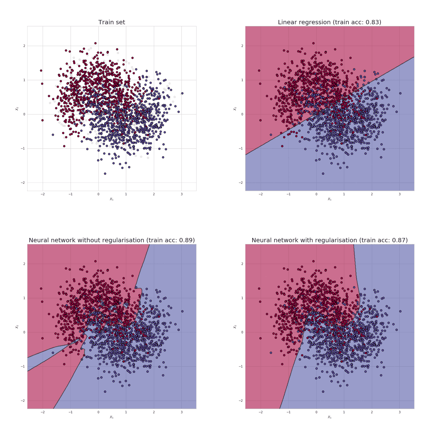
One of the most important aspects when training neural network is avoiding overfitting and also one of the most common problems data science professionals face. Have you come across a situation where your model performed exceptionally well on train data but was not able to predict test data.

Have you seen this image before? As we move towards the right in this image, our model tries to learn too well the details and the noise from the training data, which ultimately results in poor performance on the unseen data.
In other words, while going towards the right, the complexity of the model increases such that the training error reduces but the testing error doesn’t. This is shown in the image below. Overfitting refers to the phenomenon where a neural network models the training data very well but fails when it sees new data from the same problem. Overfitting is caused by noise in the training data that the neural network picks up during training and learns it as an underlying concept of the data. The model on the right side above is with a high complexity is able to pick up and learn patterns even noise in the data that are just caused by some random fluctuation or error.
On the other hand, the lower complexity network on the left side models the distribution much better by not trying too hard to model each data pattern individually.

Overfitting causes the neurla network model to perform very well during training phase but the performance gets much worse during inference time whrn faced with new data. Less complex neural networks are less susceptible to overfitting. To prevent overfitting or a high variance we must use something
A universal problem in machine learning has been making an algorithm that performs equally well on training data and any new samples or test dataset. Techniques used in machine learning that have specifically been designed to cater to reducing test error, mostly at the expense of increased training error, are globally known as regularization.
Regularization is a technique which makes slight modifications to the learning algorithm such that the model generalizes better. This in turn improves the model’s performance on the unseen data as well.
Regularization may be defined as any modification or change in the learning algorithm that helps reduce its error over a test dataset, commonly known as generalization error but not on the supplied or training dataset.
In learning algorithms, there are many variants of regularization techniques, each of which tries to cater to different challenges. These can be listed down straightforwardly based on the kind of challenge the technique is trying to deal with:
- Some try to put extra constraints on the learning of an ML model, like adding restrictions on the range/type of parameter values.
- Some add more terms in the objective or cost function, like a soft constraint on the parameter values. More often than not, a careful selection of the right constraints and penalties in the cost function contributes to a massive boost in the model's performance, specifically on the test dataset.
- These extra terms can also be encoded based on some prior information that closely relates to the dataset or the problem statement.
- One of the most commonly used regularization techniques is creating ensemble models, which take into account the collective decision of multiple models, each trained with different samples of data.
The main aim of regularization is to reduce the over-complexity of the machine learning models and help the model learn a simpler function to promote generalization.
In order to understand how the deviation of the function is varied, bias and variance can be adopted. Bias is the measurement of deviation or error from the real value of function (Train data), variance is the measurement of deviation in the response variable function while estimating it over a different training sample of the dataset (Test Data)
Therefore, for a generalized data model, we must keep bias possibly low while modelling that leads to high accuracy. And, one should not obtain greatly varied results from output, therefore, low variance is recommended for a model to perform good.
The underlying association between bias and variance is closely related to the overfitting, underfitting and capacity in machine learning such that while calculating the generalization error (where bias and variance are crucial elements) increase in the model capacity can lead to increase in variance and decrease in bias.
The trade-off is the tension amid error introduced by the bias and the variance.
Bias vs variance tradeoff graph here sheds a bit more light on the nuances of this topic and demarcation:


Regularization of an estimator works by trading increased bias for reduced variance. An effective regularize will be the one that makes the best trade between bias and variance, and the end-product of the tradeoff should be a significant reduction in variance at minimum expense to bias. In simpler terms, this would mean low variance without immensely increasing the bias value.
Let’s consider a neural network which is overfitting on the training data as shown in the image below.

If you have studied the concept of regularization in machine learning, you will have a fair idea that regularization penalizes the coefficients. In deep learning, it actually penalizes the weight matrices of the nodes.
Assume that our regularization coefficient is so high that some of the weight matrices are nearly equal to zero.

This will result in a much simpler linear network and slight underfitting of the training data.
Such a large value of the regularization coefficient is not that useful. We need to optimize the value of regularization coefficient in order to obtain a well-fitted model as shown in the image below.

Now that we have an understanding of how regularization helps in reducing overfitting, we’ll learn a few different techniques in order to apply regularization in deep learning.
L1 and L2 are the most common types of regularization. These update the general cost function by adding another term known as the regularization term.
Cost function = Loss (say, binary cross entropy) + Regularization term
Due to the addition of this regularization term, the values of weight matrices decrease because it assumes that a neural network with smaller weight matrices leads to simpler models. Therefore, it will also reduce overfitting to quite an extent.
However, this regularization term differs in L1 and L2.
The Regression model that uses L2 regularization is called Ridge Regression.


Regularization adds the penalty as model complexity increases. The regularization parameter (lambda) penalizes all the parameters except intercept so that the model generalizes the data and won’t overfit. Ridge regression adds “squared magnitude of the coefficient” as penalty term to the loss function. Here the box part in the above image represents the L2 regularization element/term.
Lambda is a hyperparameter.
If lambda is zero, then it is equivalent to OLS.
Ordinary Least Square or OLS, is a stats model which also helps us in identifying more significant features that can have a heavy influence on the output.
But if lambda is very large, then it will add too much weight, and it will lead to under-fitting. Important points to be considered about L2 can be listed below:
- Ridge regularization forces the weights to be small but does not make them zero and does not give the sparse solution.
- Ridge is not robust to outliers as square terms blow up the error differences of the outliers, and the regularization term tries to fix it by penalizing the weights.
- Ridge regression performs better when all the input features influence the output, and all with weights are of roughly equal size.
- L2 regularization can learn complex data patterns
Here, lambda is the regularization parameter. It is the hyperparameter whose value is optimized for better results. L2 regularization is also known as weight decay as it forces the weights to decay towards zero (but not exactly zero).
Lasso Regression (Least Absolute Shrinkage and Selection Operator) adds “Absolute value of magnitude” of coefficient, as penalty term to the loss function.
Lasso shrinks the less important feature’s coefficient to zero; thus, removing some feature altogether. So, this works well for feature selection in case we have a huge number of features.


L1 regularization is that it is easy to implement and can be trained as a one-shot thing, meaning that once it is trained you are done with it and can just use the parameter vector and weights.L1 regularization is robust in dealing with outliers. It creates sparsity in the solution (most of the coefficients of the solution are zero), which means the less important features or noise terms will be zero. It makes L1 regularization robust to outliers.
To understand the above mentioned point, let us go through the following example and try to understand what it means when an algorithm is said to be sensitive to outliers
- For instance we are trying to classify images of various birds of different species and have a neural network with a few hundred parameters.
- We find a sample of birds of one species, which we have no reason to believe are of any different species from all the others.
- We add this image to the training set and try to train the neural network. This is like throwing an outlier into the mix of all the others. By looking at the edge of the hyperspace where the hyperplane is closest to, we pick up on this outlier, but by the time we’ve got to the hyperplane it’s quite far from the plane and is hence an outlier.
- The solution in such cases is to perform iterative dropout. L1 regularization is a one-shot solution, but in the end we are going to have to make some kind of hard decision on where to cut off the edges of the hyperspace.
- Iterative dropout is a method of deciding exactly where to cut off. It is a little more expensive in terms of training time, but in the end it might give us an easier decision about how far the hyperspace edges are.
Along with shrinking coefficients, the lasso performs feature selection, as well. (Remember the ‘selection‘ in the lasso full-form?) Because some of the coefficients become exactly zero, which is equivalent to the particular feature being excluded from the model.
In this, we penalize the absolute value of the weights. Unlike L2, the weights may be reduced to zero here. Hence, it is very useful when we are trying to compress our model. Otherwise, we usually prefer L2 over it.


Smaller weights reduce the impact of the hidden neurons. In that case, those neurons becomes negligible and the overall complexity of the neural network gets reduced.
But we have to be careful. When chossing the regularization term
If our $alpha$ value is to high, our model is too simple, but you run the risk of underfitting our data. Our model won't learn enough about the training data to make useful predictions.If our $alpha$ value is too low, our model will be more complex and we run to the risk of overfitting our data. Our model will learn too much about the particularities of the training data will even pick up the noise in the data and then the model won't even be able to generalize to new data.
Dropout is implemented per-layer in a neural network.
It can be used with most types of layers, such as dense fully connected layers, convolutional layers, and recurrent layers such as the long short-term memory network layer.
Dropout may be implemented on any or all hidden layers in the network as well as the visible or input layer. It is not used on the output layer.
Dropout is not used after training when making a prediction with the fit network.
The weights of the network will be larger than normal because of dropout. Therefore, before finalizing the network, the weights are first scaled by the chosen dropout rate. The network can then be used as per normal to make predictions.
If a unit is retained with probability p during training, the outgoing weights of that unit are multiplied by p at test time.
The rescaling of the weights can be performed at training time instead, after each weight update at the end of the mini-batch. This is sometimes called “inverse dropout” and does not require any modification of weights during training. Both the Keras and PyTorch deep learning libraries implement dropout in this way.
At test time, we scale down the output by the dropout rate. […] Note that this process can be implemented by doing both operations at training time and leaving the output unchanged at test time, which is often the way it’s implemented in practice
Dropout works well in practice, perhaps replacing the need for weight regularization (e.g. weight decay) and activity regularization (e.g. representation sparsity).
… dropout is more effective than other standard computationally inexpensive regularizers, such as weight decay, filter norm constraints and sparse activity regularization. Dropout may also be combined with other forms of regularization to yield a further improvement.
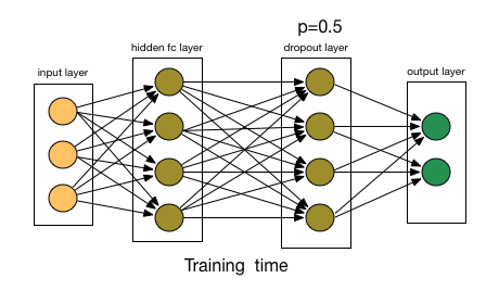
The term 'dropout' refers to dropping out units (both hidden and visible) (neurons) in a neural network. Simply put, dropout refers to ignoring units (i.e. neurons) during the training phase of certain set of neurons which is chosen at random. By “ignoring”, I mean these units are not considered during a particular forward or backward pass. At each training phase, individual nodes are either dropout of the net with probability (1-p) or kept with probability p, so that a shallow network is left (less dense)
Given that we know a bit about dropout, a question arises — why do we need dropout at all? Why do we need to literally shut-down parts of a neural networks?
A fully connected layer occupies most of the parameters and hence, neurons develop co- dependency amongst each other during training which curbs the individual power of each neuron leading to over-fitting of training data.
- Training Phase:
Training Phase: For each hidden layer, for each training sample, for each iteration, ignore (zero out) a random fraction, p, of nodes (and corresponding activations).
- Testing Phase:
Use all activations, but reduce them by a factor p (to account for the missing activations during training).

Dropout means, that during training with some probability "p" a number of neurons of the neural networks gets turned off during training.
Let say p=0.5 you can observe on right approx half of the neurons are not active.
Let’s try this theory in practice. To see how dropout works, I build a deep net in Keras and tried to validate it on the CIFAR-10 dataset. The deep network is built had three convolution layers of size 64, 128 and 256 followed by two densely connected layers of size 512 and an output layer dense layer of size 10 (number of classes in the CIFAR-10 dataset).
I took ReLU as the activation function for hidden layers and sigmoid for the output layer (these are standards, didn’t experiment much on changing these). Also, I used the standard categorical cross-entropy loss.
Finally, I used dropout in all layers and increase the fraction of dropout from 0.0 (no dropout at all) to 0.9 with a step size of 0.1 and ran each of those to 20 epochs. The results look like this:


From the above graphs we can conclude that with increasing the dropout, there is some increase in validation accuracy and decrease in loss initially before the trend starts to go down. There could be two reasons for the trend to go down if dropout fraction is 0.2:
- 0.2 is actual minima for the this dataset, network and the set parameters used
- More epochs are needed to train the networks.
This probability of choosing how many nodes should be dropped is the hyperparameter of the dropout function. As seen in the image above, dropout can be applied to both the hidden layers as well as the input layers.
This section provides some tips for using dropout regularization with your neural network.
Dropout regularization is a generic approach.
It can be used with most, perhaps all, types of neural network models, not least the most common network types of Multilayer Perceptrons, Convolutional Neural Networks, and Long Short-Term Memory Recurrent Neural Networks.
In the case of LSTMs, it may be desirable to use different dropout rates for the input and recurrent connections.
The default interpretation of the dropout hyperparameter is the probability of training a given node in a layer, where 1.0 means no dropout, and 0.0 means no outputs from the layer.
A good value for dropout in a hidden layer is between 0.5 and 0.8. Input layers use a larger dropout rate, such as of 0.8.
It is common for larger networks (more layers or more nodes) to more easily overfit the training data.
When using dropout regularization, it is possible to use larger networks with less risk of overfitting. In fact, a large network (more nodes per layer) may be required as dropout will probabilistically reduce the capacity of the network.
A good rule of thumb is to divide the number of nodes in the layer before dropout by the proposed dropout rate and use that as the number of nodes in the new network that uses dropout. For example, a network with 100 nodes and a proposed dropout rate of 0.5 will require 200 nodes (100 / 0.5) when using dropout.
If n is the number of hidden units in any layer and p is the probability of retaining a unit […] a good dropout net should have at least n/p units
Network weights will increase in size in response to the probabilistic removal of layer activations.
Large weight size can be a sign of an unstable network.
To counter this effect a weight constraint can be imposed to force the norm (magnitude) of all weights in a layer to be below a specified value. For example, the maximum norm constraint is recommended with a value between 3-4.
[…] we can use max-norm regularization. This constrains the norm of the vector of incoming weights at each hidden unit to be bound by a constant c. Typical values of c range from 3 to 4.
This does introduce an additional hyperparameter that may require tuning for the model.
Like other regularization methods, dropout is more effective on those problems where there is a limited amount of training data and the model is likely to overfit the training data.
Problems where there is a large amount of training data may see less benefit from using dropout.
For very large datasets, regularization confers little reduction in generalization error. In these cases, the computational cost of using dropout and larger models may outweigh the benefit of regularization.
Much of the success of deep learning has come from building larger and larger neural networks. This allows these models to perform better on various tasks, but also makes them more expensive to use. Larger models take more storage space which makes them harder to distribute. Larger models also take more time to run and can require more expensive hardware. This is especially a concern if you are productionizing a model for a real-world application.
Model compression aims to reduce the size of models while minimizing loss in accuracy or performance. Neural network pruning is a method of compression that involves removing weights from a trained model. In agriculture, pruning is cutting off unnecessary branches or stems of a plant. In machine learning, pruning is removing unnecessary neurons or weights. We will go over some basic concepts and methods of neural network pruning.
As we know that an efficient model is that model which optimizes memory usage and performance at the inference time. Deep Learning model inference is just as crucial as model training, and it is ultimately what determines the solution’s performance metrics. Once the deep learning model has been properly trained for a given application, the next stage is to guarantee that the model is deployed into a production-ready environment, which requires both the application and the model to be efficient and dependable.
Maintaining a healthy balance between model correctness and inference time is critical. The running cost of the implemented solution is determined by the inference time. It’s crucial to have memory-optimized and real-time (or lower latency) models since the system where your solution will be deployed may have memory limits.
Developers are looking for novel and more effective ways to reduce the computing costs of neural networks as image processing, finance, facial recognition, facial authentication, and voice assistants all require real-time processing. Pruning is one of the most used procedures.
Pruning is the process of deleting parameters from an existing neural network, which might involve removing individual parameters or groups of parameters, such as neurons. This procedure aims to keep the network’s accuracy while enhancing its efficiency. This can be done to cut down on the amount of computing power necessary to run the neural network.

Pruning can take many different forms, with the approach chosen based on our desired output. In some circumstances, speed takes precedence over memory, whereas in others, memory is sacrificed. The way sparsity structure, scoring, scheduling, and fine-tuning are handled by different pruning approaches.

-
Structured and Unstructured Pruning
-
- Remove weights or neurons?
There are different ways to prune a neural network.
Individual parameters are pruned using an unstructured pruning approach. This results in a sparse neural network, which, while lower in terms of parameter count, may not be configured in a way that promotes speed improvements.
Randomly zeroing out the parameters saves memory but may not necessarily improve computing performance because we end up conducting the same number of matrix multiplications as before.
Because we set specific weights in the weight matrix to zero, this is also known as Weight Pruning.
(1) You can prune weights. This is done by setting individual parameters to zero and making the network sparse. This would lower the number of parameters in the model while keeping the architecture the same.
Weight-based pruning is more popular as it is easier to do without hurting the performance of the network. However, it requires sparse computations to be effective. This requires hardware support and a certain amount of sparsity to be efficient.
(2) You can remove entire nodes from the network. This would make the network architecture itself smaller, while aiming to keep the accuracy of the initial larger network.
Pruning nodes will allow dense computation which is more optimized. This allows the network to be run normally without sparse computation. This dense computation is more often better supported on hardware. However, removing entire neurons can more easily hurt the accuracy of the neural network.
A major challenge in pruning is determining what to prune. If you are removing weights or nodes from a model, you want the parameters you remove to be less useful. There are different heuristics and methods of determining which nodes are less important and can be removed with minimal effect on accuracy. You can use heuristics based on the weights or activations of a neuron to determine how important it is for the model’s performance. The goal is to remove more of the less important parameters.
One of the simplest ways to prune is based on the magnitude of the weight. Removing a weight is essentially setting it to zero. You can minimize the effect on the network by removing weights that are already close to zero, meaning low in magnitude. This can be implemented by removing all weights below a certain threshold. To prune a neuron based on weight magnitude you can use the L2 norm of the neuron’s weights.
Rather than just weights, activations on training data can be used as a criteria for pruning. When running a dataset through a network, certain statistics of the activations can be observed. You may observe that some neurons always outputs near-zero values. Those neurons can likely be removed with little impact on the model. The intuition is that if a neuron rarely activates with a high value, then it is rarely used in the model’s task.
In addition to the magnitude of weights or activations, redundancy of parameters can mean a neuron can be removed. If two neurons in a layer have very similar weights or activations, it can mean they are doing the same thing. By this intuition, we can remove one of the neurons and preserve the same functionality.
Ideally in a neural network, all the neurons have unique parameters and output activations that are significant in magnitude and not redundant. We want all the neurons are doing something unique, and remove those that are not.
A major consideration in pruning is where to put it in the training/testing machine learning timeline. If you are using a weight magnitude-based pruning approach, as described in the previous section, you would want to prune after training. However, after pruning, you may observe that the model performance has suffered. This can be fixed by fine-tuning, meaning retraining the model after pruning to restore accuracy.

The usage of pruning can change depending on the application and methods used. Sometimes fine-tuning or multiple iterations of pruning are not necessary. This depends on how much of the network is pruned.
There multiple metrics to consider when evaluating a pruning method: accuracy, size, and computation time. Accuracy is needed to determine how the model performs on its task. Model size is how much bytes of storage the model takes. To determine computation time, you can use FLOPs (Floating point operations) as a metric. This is more consistent to measure than inference time and it does not depend on what system the model runs on.
With pruning, there is a tradeoff between model performance and efficiency. You can prune heavily and have a smaller more efficient network, but also less accurate. Or you could prune lightly and have a highly performant network, that is also large and expensive to operate. This trade-off needs to be considered for different applications of the neural network.
- Determine the significance of each neuron.
- Prioritize the neurons based on their value (assuming there is a clearly defined measure for “importance”).
- Remove the neuron that is the least significant.
- Determine whether to prune further based on a termination condition (to be defined by the user).
- If unanticipated adjustments in data distribution may occur during deployment, don’t prune.
- If you only have a partial understanding of the distribution shifts throughout training and pruning, prune moderately.
- If you can account for all movements in the data distribution throughout training and pruning, prune to the maximum extent possible.
- When retraining, specifically consider data augmentation to maximize the prune potential.
Early stopping is a kind of cross-validation strategy where we keep one part of the training set as the validation set. When we see that the performance on the validation set is getting worse, we immediately stop the training on the model. This is known as early stopping.

In the above image, we will stop training at the dotted line since after that our model will start overfitting on the training data.
In keras, we can apply early stopping using the callbacks function. Below is the sample code for it.

Here, monitor denotes the quantity that needs to be monitored and ‘val_err’ denotes the validation error.
Patience denotes the number of epochs with no further improvement after which the training will be stopped. For better understanding, let’s take a look at the above image again. After the dotted line, each epoch will result in a higher value of validation error. Therefore, 5 epochs after the dotted line (since our patience is equal to 5), our model will stop because no further improvement is seen.
Note: It may be possible that after 5 epochs (this is the value defined for patience in general), the model starts improving again and the validation error starts decreasing as well. Therefore, we need to take extra care while tuning this hyperparameter.
Training a neural network consists of the following basic steps:
-
Step-1: Initialization of Neural Network: Initialize weights and biases.
-
Step-2: Forward propagation: Using the given input X, weights W, and biases b, for every layer we compute a linear combination of inputs and weights (Z)and then apply activation function to linear combination (A). At the final layer, we compute f(A(l-1)) which could be a sigmoid (for binary classification problem), softmax (for multi-class classification problem), and this gives the prediction y_hat.
-
Step-3: Compute the loss function: The loss function includes both the actual label y and predicted label y_hat in its expression. It shows how far our predictions from the actual target, and our main objective is to minimize the loss function.
-
Step-4: Backward Propagation: In backpropagation, we find the gradients of the loss function, which is a function of y and y_hat, and gradients wrt A, W, and b called dA, dW, and db. By using these gradients, we update the values of the parameters from the last layer to the first layer.
-
Step-5: Repeat steps 2–4 for n epochs till we observe that the loss function is minimized, without overfitting the train data.
For Example,
For a neural network having 2 layers, i.e. one hidden layer. (Here bias term is not added just for the simplicity)


- 1.) In the first step, Input units are passed i.e data is passes with some weights attached to it to the hidden layers. WE can have any number of hidden layers.
- 2.) Each hidden layers consists of neurons. All the inputs are connected to neuron (each).
- 3.) After passing on the inputs, all the the computation is performed in the hidden layers.
Computation performed in hidden layers are done in two steps which are as follows:-
First of all, all the inputs are multiplied by their respective weights assigned. Weights are the gradient of each variable. It shows the strength of the particular input. After assigning the weights, a bias variable is added. Bias is coefficient of each variable and it is constant that helps the model to fit in the best way possible.
Then in the second step, the activation function is applied to the linear equation 'y'. The activation function is a non-linear transformation that is applied to the input before sending it to the next layer of neuron. The importance of the activation function is to incubate non-linearity i the model.
The whole process described in point 3 is performed in each hidden layers. After passing through every hidden layers we move to the last layer i.e our output layer which gives us the final output.
After getting the predictions from the output layers, the error is calculated i.e the difference between the actual and the predicted output. If the error is large then steps are take to minimize the error and for the same purpose Back propogation is performed.
Artificial Neural Network (ANN) are comprised of node layers. containing an input layer, one or more hidden layers, and a output layer. Each node or artificial neuron, connects to another and has an associated weigths and threshold.
If the output of any individual node is above the specified threshold value, that ndoe is activated, sending data to the next layer of the network otherwise, no data is passed along to the next layer of the network.
Once an input layer is determined, weight are assigned. These weights help determine the importance of any given variable, with larger ones contributing more significantly to the output compared to other inputs
All inputs are then multiplied by their respective weights and then summed. Afterwards, the output is passed through an activation function, which determines the output. If the ouput exceeds a given threshold, it 'fires' (or activates) the node, passing data to the next layer in the network. This results in the output of one node becoming in the input of the next node.

|