Covid-Job-Loss-Econmetrics-Project

This is a project done in Stata, for an econometrics class. The goal of the project was to show how job retention was different in rural vs urban areas during the early stages of the Covid-19 pandemic.

Introduction

The topic of discussion in this paper is primarily whether those who live in metro areas experienced significantly greater likelihood of job-loss due to covid (from here on JLDC) than those living outside of such areas. This comparison will be made considering state fixed effects, age, gender, and race. Following this, what will be determined is if there is a notable difference in JLDC in metro areas depending on whether an individual is employed by a for-profit company, a non-profit, or the government. This is important, because with a lot of JLDC across the country, there is a large portion of the labor force that was underutilized over the past year. So long as they could be kept safe at work, it would help the economy in the event of another pandemic to have some of those people working for non-profits or the government to contribute to GDP and to do things such as distribute the vaccine or help keep our public spaces clean of the virus. This would be more likely possible if those with government jobs, and in the non-profit sector were able to have a lower likelihood of JLDC. Finally, it will be determined if controlling for those who teleworked, they experienced less likelihood of JDLC within the cities than outside of them. This is an important question to answer because it will show if the measures taken to allow remote work succeeded in decreasing job loss in metro areas, where covid-19 related joblessness is bound to be higher due to a higher population being in a denser area. With this question answered, we will know in the event of a future pandemic if supporting businesses in providing opportunities to work remotely in bigger cities would be an effective way to curb job loss. It should be noted, that the benchmark for statistical significance that will be used for my purposes will be the 5% level, so that will be the determinant of whether or not there are significant differences in the groups specified above.

The Models

In each regression that I ran, I chose to include an age2 group, since I believe age an inability to work due to covid is not a straight linear relationship, and instead would be represented better by a polynomial regression. The first model I built was a regression of age, gender, education, and race on a binary variable that was equal to one if an individual was unable to work due to covid and zero otherwise. This first regression also accounted for state fixed effects, so as to account for regional differences in metro and rural areas between states. The model broken down looks like:

$$𝐽𝐿𝐷𝐶 ̂= 𝛼 ̂+𝛽̂0∗𝑆𝑡𝑎𝑡𝑒1−50+𝛽̂1∗𝑀𝑒𝑡𝑟𝑜+𝛽̂2∗𝐴𝑔𝑒+𝛽̂3∗𝐴𝑔𝑒2+𝛽̂4∗𝑆𝑒𝑥 + 𝛽̂5∗𝐻𝑖𝑠𝑝𝑎𝑛𝑖𝑐+ 𝛽̂6∗𝐵𝑙𝑎𝑐𝑘+$$ $$𝛽̂7∗𝐴𝑠𝑖𝑎𝑛+𝛽̂8∗𝑂𝑡ℎ𝑒𝑟𝑅𝑎𝑐𝑒+𝛽̂9∗𝑆𝑜𝑚𝑒𝐶𝑜𝑙𝑙𝑒𝑔𝑒+ 𝛽̂10∗𝐵𝑎𝑐ℎ𝑒𝑙𝑜𝑟𝑠+ 𝛽̂11∗𝑀𝑎𝑠𝑡𝑒𝑟𝑠𝑃𝑙𝑢𝑠$$

To keep things simple, I combined groups from different parts of the metro area into one grouping and compared it to those outside of the metro area. There was data available on people in the inner-city part of a metro area versus not as well, however that didn’t seem to add a lot to the model and served to cause other problems within Stata when I added state fixed effects, so this simplification was made. The second regression I ran was based on the first, but also included several dummy variables for each “class” of worker to determine if there are significant differences between what the model predicts should be the JLDC for non-profit, versus for-profit, versus government jobs, while still accounting for the control variables from the first regression. The model used for the second regression is as follows:

$$𝐽𝐿𝐷𝐶 ̂= 𝛼 ̂+𝛽̂0∗𝑆𝑡𝑎𝑡𝑒1−50+𝛽̂1∗𝑀𝑒𝑡𝑟𝑜+𝛽̂2∗𝐴𝑔𝑒+𝛽̂3∗𝐴𝑔𝑒2+𝛽̂4∗𝑆𝑒𝑥 + 𝛽̂5∗𝐻𝑖𝑠𝑝𝑎𝑛𝑖𝑐+ 𝛽̂6∗𝐵𝑙𝑎𝑐𝑘+$$ $$𝛽̂7∗𝐴𝑠𝑖𝑎𝑛+𝛽̂8∗𝑂𝑡ℎ𝑒𝑟𝑅𝑎𝑐𝑒+ 𝛽̂9∗𝑆𝑜𝑚𝑒𝐶𝑜𝑙𝑙𝑒𝑔𝑒+ 𝛽̂10∗𝐵𝑎𝑐ℎ𝑒𝑙𝑜𝑟𝑠+ 𝛽̂11∗𝑀𝑎𝑠𝑡𝑒𝑟𝑠𝑃𝑙𝑢𝑠 + 𝛽̂12∗𝑆𝑒𝑙𝑓𝐸𝑚𝑝𝑙𝑜𝑦𝑒𝑑 +$$ $$𝛽̂13∗𝑁𝑜𝑛𝑃𝑟𝑜𝑓𝑖𝑡𝐸𝑚𝑝𝑙𝑜𝑦𝑒𝑑+ 𝛽̂14∗𝐺𝑜𝑣𝑒𝑟𝑛𝑚𝑒𝑛𝑡𝐸𝑚𝑝𝑙𝑜𝑦𝑒d$$

For this model, in order to avoid perfect multicollinearity, the reference group used was the group that was employed by a for-profit company. This decision was made because I believed it would show greater clearer differences between the for-profit and the non-profit and government jobs, than if I had used the self-employed category. The final model that was used looked at JLDC was based on the second one outlined above, and then modified to include dummy variable for working remotely. It is as follows:

$$𝐽𝐿𝐷𝐶 ̂= 𝛼 ̂+𝛽̂0∗𝑆𝑡𝑎𝑡𝑒1−50+𝛽̂1∗𝑀𝑒𝑡𝑟𝑜+𝛽̂2∗𝐴𝑔𝑒+𝛽̂3∗𝐴𝑔𝑒2+𝛽̂4∗𝑆𝑒𝑥 + 𝛽̂5∗𝐻𝑖𝑠𝑝𝑎𝑛𝑖𝑐+ 𝛽̂6∗𝐵𝑙𝑎𝑐𝑘+$$ $$𝛽̂7∗𝐴𝑠𝑖𝑎𝑛+𝛽̂8∗𝑂𝑡ℎ𝑒𝑟𝑅𝑎𝑐𝑒+ 𝛽̂9∗𝑆𝑜𝑚𝑒𝐶𝑜𝑙𝑙𝑒𝑔𝑒+ 𝛽̂10∗𝐵𝑎𝑐ℎ𝑒𝑙𝑜𝑟𝑠+ 𝛽̂11∗𝑀𝑎𝑠𝑡𝑒𝑟𝑠𝑃𝑙𝑢𝑠 + 𝛽̂12∗𝑆𝑒𝑙𝑓𝐸𝑚𝑝𝑙𝑜𝑦𝑒𝑑 +$$ $$𝛽̂13∗𝑁𝑜𝑛𝑃𝑟𝑜𝑓𝑖𝑡𝐸𝑚𝑝𝑙𝑜𝑦𝑒𝑑+ 𝛽̂14∗𝐺𝑜𝑣𝑒𝑟𝑛𝑚𝑒𝑛𝑡𝐸𝑚𝑝𝑙𝑜𝑦𝑒𝑑 + 𝛽̂15∗𝑅𝑒𝑚𝑜𝑡𝑒+ 𝛽̂16∗𝑅𝑒𝑚𝑜𝑡𝑒And𝑀𝑒𝑡𝑟𝑜$$

I also chose to include the interaction term for instances where people lived in the city and worked remotely, since I thought this would be significant since teleworking has been more common in cities, where there is a larger population.

The Data

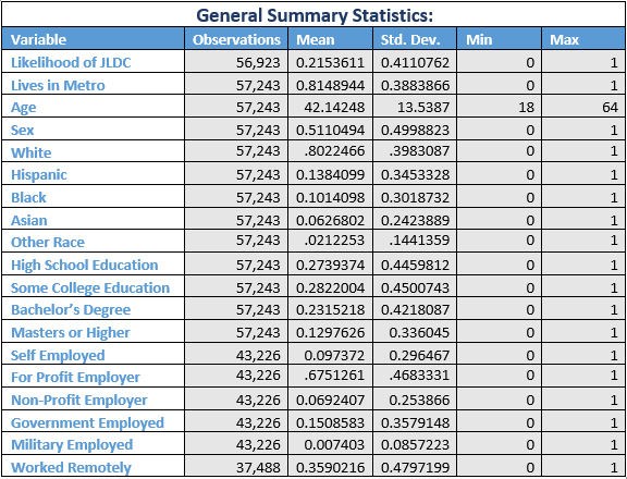
Included in my models as the reference groups for the dummy variables were the white group, the high school education group, and the for-profit employed group. I also excluded those who’s data did not have information for the likelihood of JLDC, race, class of employment, and remote work status in each relevant regression above. This, however, I do not believe skewed my results, since there were still over 37,473 observations of individuals who did have data in those categories; even in the one which I had to drop the highest number of observations.

The Results

For the results, I will start by reiterating the models above, but filling in the coefficients to show the estimates I got in my results. Then I will outline how and if they differ from what I expected.

Model 1

$$𝐽𝐿𝐷𝐶 ̂= 𝛼 ̂+𝟎.𝟎𝟏𝟔𝟐∗𝑀𝑒𝑡𝑟𝑜+0.00565∗𝐴𝑔𝑒+−0.00008∗𝐴𝑔𝑒2+0.0115∗𝑆𝑒𝑥 + 0.0550∗𝐻𝑖𝑠𝑝𝑎𝑛𝑖𝑐+ 0.0208∗𝐵𝑙𝑎𝑐𝑘+$$ $$0.0259∗𝐴𝑠𝑖𝑎𝑛+0.0256∗𝑂𝑡ℎ𝑒𝑟𝑅𝑎𝑐𝑒+0.00909∗𝑆𝑜𝑚𝑒𝐶𝑜𝑙𝑙𝑒𝑔𝑒+ −0.0452∗𝐵𝑎𝑐ℎ𝑒𝑙𝑜𝑟𝑠+ −0.0878∗𝑀𝑎𝑠𝑡𝑒𝑟𝑠𝑃𝑙𝑢𝑠$$

In this initial model, I started out simply determining whether there was a significant difference in job loss according to this data between those living inside and outside of metro areas. Living in a metro area was found to be only statistically significant at the 5% level, which was less significant than I had expected, since I assumed that the larger population in metro areas and cramped living conditions would be a large contributing factor in JLDC. My results show that living in a metro area is associated with a 1.62% increase in the likelihood of JLDC. This means that those living outside of metro areas were less likely to experience JLDC when controlling for age, sex, race, and education.

Model 2

$$𝐽𝐿𝐷𝐶 ̂= 𝛼 ̂+0.0162∗𝑀𝑒𝑡𝑟𝑜+0.00565∗𝐴𝑔𝑒+−0.00008∗𝐴𝑔𝑒2+0.0115∗𝑆𝑒𝑥 + 0.0550∗𝐻𝑖𝑠𝑝𝑎𝑛𝑖𝑐+ 0.0208∗𝐵𝑙𝑎𝑐𝑘+$$ $$0.0259∗𝐴𝑠𝑖𝑎𝑛+0.0256∗𝑂𝑡ℎ𝑒𝑟𝑅𝑎𝑐𝑒+0.00909∗𝑆𝑜𝑚𝑒𝐶𝑜𝑙𝑙𝑒𝑔𝑒+ −0.0452∗𝐵𝑎𝑐ℎ𝑒𝑙𝑜𝑟𝑠+ −0.0878∗𝑀𝑎𝑠𝑡𝑒𝑟𝑠𝑃𝑙𝑢𝑠 +$$ $$0.180∗𝑆𝑒𝑙𝑓𝐸𝑚𝑝𝑙𝑜𝑦𝑒𝑑 + −𝟎.𝟎𝟑𝟖𝟏∗𝑁𝑜𝑛𝑃𝑟𝑜𝑓𝑖𝑡𝐸𝑚𝑝𝑙𝑜𝑦𝑒𝑑+ −0.0673∗𝐺𝑜𝑣𝑒𝑟𝑛𝑚𝑒𝑛𝑡𝐸𝑚𝑝𝑙𝑜𝑦𝑒d$$

Within this model, I added dummy variables for different “classes” of employment which would represent the different types of employer a person could have. Interestingly, controlling for employment made living in a metro area no longer statistically significant at the 5% level, which I believe is an artifact of the standard error for lives in metro being greatly reduced by this change. When I ran an F-test on the variables I added to the model this time, the p value showed that these variables are statistically significant. I found that working for a non-profit is associated with a 3.81% decrease in the likelihood of JLDC compared to working for a for-profit company (controlling for race, age, sex, and education). This itself was significant at the 1% level in this model, which initially gave me the idea that this was a good indicator that my model was representing the difference in for-profit and non-for profit companies, however that notion was quickly challenged by the results of the final model.

Model 3

$$𝐽𝐿𝐷𝐶 ̂= 𝛼 ̂+0.0418∗𝑀𝑒𝑡𝑟𝑜+ −0.00359∗𝐴𝑔𝑒+ 0.0000323∗𝐴𝑔𝑒2+0.0467∗𝑆𝑒𝑥 + 0.0415∗𝐻𝑖𝑠𝑝𝑎𝑛𝑖𝑐+ 0.0171∗𝐵𝑙𝑎𝑐𝑘+$$ $$0.0196∗𝐴𝑠𝑖𝑎𝑛+ 0.00595∗𝑂𝑡ℎ𝑒𝑟𝑅𝑎𝑐𝑒+ −0.00822∗𝑆𝑜𝑚𝑒𝐶𝑜𝑙𝑙𝑒𝑔𝑒+ −0.0522∗𝐵𝑎𝑐ℎ𝑒𝑙𝑜𝑟𝑠+ −0.0645∗𝑀𝑎𝑠𝑡𝑒𝑟𝑠𝑃𝑙𝑢𝑠 + 0.220∗𝑆𝑒𝑙𝑓𝐸𝑚𝑝𝑙𝑜𝑦𝑒𝑑 +$$ $$−0.0172∗𝑁𝑜𝑛𝑃𝑟𝑜𝑓𝑖𝑡𝐸𝑚𝑝𝑙𝑜𝑦𝑒𝑑+ −0.0451∗𝐺𝑜𝑣𝑒𝑟𝑛𝑚𝑒𝑛𝑡𝐸𝑚𝑝𝑙𝑜𝑦𝑒𝑑 + 𝟎.𝟎𝟔𝟏𝟗∗𝑅𝑒𝑚𝑜𝑡𝑒+ −𝟎.𝟏𝟎𝟗∗𝑅𝑒𝑚𝑜𝑡𝑒And𝑀𝑒𝑡𝑟𝑜$$

In the last model I created, I added even more dummy variables to see the effect of working remotely, as well as working remotely while living in a metro area, had on likelihood of JLDC. Both the f-test for joint significance, as well as the individual p-values for working remotely as well as working remotely while living in a metro area were statistically significant at the 1% level. Working remotely while living in a rural area was associated with a 6.19% increase in the likelihood of JLDC and working remotely while living in a metro area was associated with a 10.9% decrease in the likelihood of JLDC. There is a stark departure in how the two different types of area differ in how well they can continue to support remote work compared each other. As referenced above, in the section detailing the results of the second model, this addition to the model made it so that the results showed that working for a non-profit was not statistically significantly different from working for a for-profit once you control for remote working.

Conclusion

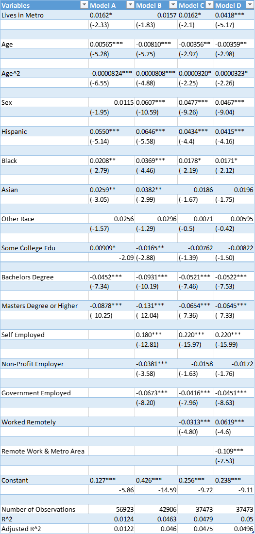
All the data considered; I believe my final model ended up being the most accurate of the three. As I added more variables into the model, the significance of factors such as race shrank with each iteration, and the significance of factors such as sex and living in a metro area grew in significance. It would be interesting to go back and test out more interaction terms to the model between working remotely and other variables, because I believe my results indicate that women working remotely may differ significantly from me when it comes to likelihood of JLDC. The main takeaway from my results personally was from the final model, where I found that not only are those in metro areas associated with a 10% reduction in likelihood of JLDC, but also those who live in rural areas also experience a nearly 7% increase in likelihood of JLDC. This makes it apparent to me that in the event of another such tragedy as a pandemic like this, it might be a good idea to provide other solutions for those living outside of metro areas than remote work, since it doesn’t seem like it increases the likelihood of job retention for them. Also, remote work does seem to work in helping prevent JLDC since it associated with a decrease in the likelihood of it. Potential omitted variables include taking into account time fixed effects if that were feasible for a dataset this large, as well as variables to represent the individual levels of covid-risk for each person.