PreQual (dtiQA v7 Multi) User Guide

Overview

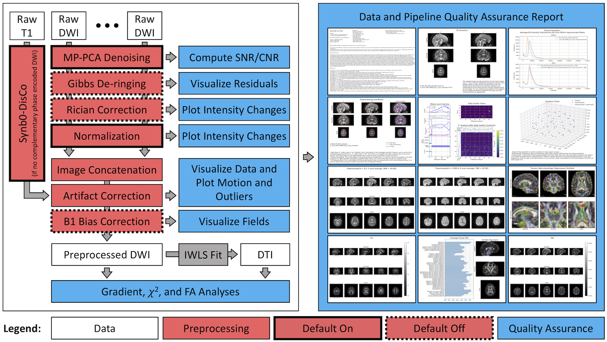
Summary: Perform integrated preprocessing and quality assurance of diffusion MRI data
Preprocessing Steps:
1. MP-PCA denoising (default on)
2. Gibbs de-ringing (default off)
3. Rician correction (default off)
4. Inter-scan normalization (default on)
5. Susceptibility-induced distortion correction, with or without reverse gradient images or field maps
6. Eddy current-induced distortion correction
7. Inter-volume motion correction
8. Slice-wise signal dropout imputation
9. N4 B1 bias field correction (default off)
10. Gradient nonlinearity correction (default off)
Quality Assurance Steps:
1. Verification of phase encoding schemes
2. Analysis of gradient directions
3. Shell-wise analysis of signal-to-noise and contrast-to-noise ratios
4. Visualization of Gibbs de-ringing changes (if applicable)
5. Visualization of within brain intensity distributions before and after Rician correction (if applicable)
6. Correction (if applicable) or visualization of inter-scan intensity relationships
7. Shell-wise analysis of distortion corrections
8. Analysis of inter-volume motion and slice-wise signal dropout
9. Analysis of B1 bias fields (if applicable)
10. Analysis of gradient nonlinear fields (if applicable)
11. Verification of intra-pipeline masking
12. Analysis of tensor goodness-of-fit
13. Voxel-wise and region-wise quantification of FA
14. Voxel-wise quantification of MD

Authors and Reference

Leon Y. Cai, Qi Yang, Colin B. Hansen, Vishwesh Nath, Karthik Ramadass, Graham W. Johnson, Benjamin N. Conrad, Brian D. Boyd, John P. Begnoche, Lori L. Beason-Held, Andrea T. Shafer, Susan M. Resnick, Warren D. Taylor, Gavin R. Price, Victoria L. Morgan, Baxter P. Rogers, Kurt G. Schilling, Bennett A. Landman. PreQual: An automated pipeline for integrated preprocessing and quality assurance of diffusion weighted MRI images. Magnetic Resonance in Medicine, 2021.

Medical-image Analysis and Statistical Interpretation (MASI) Lab, Vanderbilt University, Nashville, TN, USA

Getting Started

The PreQual software is designed to run inside a Singularity container. The container requires an "inputs" folder that holds all required input diffusion image files (i.e., .nii.gz, .bval, and .bvec files) and a configuration file. For those running Synb0-DisCo to correct susceptibility distortions without reverse phase-encoded images, this folder will also contain the structural T1 image. The container also requires an "outputs" folder that will hold all the outputs after the pipeline runs. We also need to know the image axis on which phase encoding was performed for all inputs (i.e., "i" for the first dimension, "j" for the second). To build the configuration file, we need to know the direction along said axis in which each image was phase encoded (i.e., "+" for positive direction and "-" for the negative direction) and the readout time for each input image. Once we have this information, we bind the inputs and outputs directories into the container to run the pipeline.

Note: The phase encoding axis, direction, and readout time must be known ahead of time, as this information is not stored in NIFTI headers. Depending on the scanner used, they may be available in JSON sidecars when NIFTIs are converted from DICOMs with dcm2niix.

Containerization of Source Code

git clone https://github.com/MASILab/PreQual.git
cd /path/to/repo/PreQual
git checkout v1.1.0
sudo singularity build /path/to/prequal.simg Singularity

We use Singularity version 3.8 CE with root permissions.

Alternatively, a pre-built container can be downloaded here.

Command

singularity run 
-e 
--contain
--home /path/to/inputs/directory/
-B /path/to/inputs/directory/:/INPUTS
-B /path/to/outputs/directory/:/OUTPUTS
-B /tmp:/tmp
-B /path/to/freesurfer/license.txt:/APPS/freesurfer/license.txt
-B /path/to/cuda:/usr/local/cuda
--nv
/path/to/prequal.simg
pe_axis
[options]

Binding the freesurfer license is optional and only needed for Synb0-DisCo
Binding the tmp directory is necessary when running the image with --contain.
Binding --home is necessary for matlab since it uses home for temp storage.
--nv and -B /path/to/cuda:/usr/local/cuda are optional. See options --eddy_cuda and --eddy_extra_args. GPU support is currently experimental.

Arguments and I/O

Input Directory: The dtiQA_config.csv configuration file and at least one diffusion weighted image must be provided.
- dtiQA_config.csv (see below for format, must be named exactly)
- <image1>.nii.gz (diffusion weighted image)
- <image1>.bval (units of s/mm², in the FSL format)
- <image1>.bvec (normalized unit vectors in the FSL format)
  
  :
- <imageN>.nii.gz (diffusion weighted image)
- <imageN>.bval (units of s/mm², in the FSL format)
- <imageN>.bvec (normalized unit vectors in the FSL format)
- t1.nii.gz (Optional, used for Synb0-DisCo, must be named exactly)
- gradtensor.nii (Optional, used for --correct_grad, must be named exactly)
- Other files as needed (see --extra_eddy_args for more information)
Output Directory: Full outputs listed at the end of this document
- The output preprocessed images are available in the PREPROCESSED subfolder in the output directory:
  - PREPROCESSED/dwmri.nii.gz
  - PREPROCESSED/dwmri.bval
  - PREPROCESSED/dwmri.bvec
- The QA document is available in the PDF subfolder in the output directory:
  - PDF/dtiQA.pdf
pe_axis: Phase encoding axis of all the input images. We do NOT support different phase encoding axes between different input images at this time. The options are i and j and correspond to the first and second dimension of the input images, respectively. Note that FSL does not currently support phase encoding in the third dimension (i.e. k, the dimension in which the image slices were acquired, commonly axial for RAS and LAS oriented images). This parameter is direction AGNOSTIC. The phase encoding directions of the input images along this axis are specified in the dtiQA_config.csv file. See Configuration File and Examples for more information.

Configuration File

The format for the lines of the configuration CSV file, dtiQA_config.csv (must be named exactly), are as follows:

<image1>,pe_dir,readout_time
:
<imageN>,pe_dir,readout_time

<image> is the shared file PREFIX between the corresponding NIFTI, BVAL, and BVEC files for that particular image in the input directory (i.e., my_dwi.nii.gz/.bval/.bvec -> my_dwi). Do NOT include the path to the input directory.
pe_dir is either + or -, corresponding to the direction along the phase encoding axis (as defined by the parameter pe_axis) on which the image is phase encoded.
- Note that a combination of phase encoding axis and direction map to specific anatomical (i.e. APA, APP, etc.) directions based on the orientation of the image. So, for instance in a RAS image, an axis of j and direction of + map to APP. We infer the orientation of the image from the header of the NIFTI using nibabel tools and output the best anatomical phase encoding direction interpretation of the input direction in the PDF for QA.
readout_time is a non-negative number, the readout_time parameter required by FSL’s eddy. The absolute value of this parameter is used to scale the estimated b0 field. Note a value of 0 indicates that the images are infinite bandwidth (i.e. no susceptibility distortion). See Examples for more information.

Examples

Here are some different example combinations of pe_axis, pe_dir, and readout_time parameters and the corresponding FSL acquisition parameters lines:

pe_axis	pe_dir	readout_time	acqparams line
i	+	0.05	1, 0, 0, 0.05
j	-	0.1	0, -1, 0, 0.1

These are examples of common use cases. They also all share the same command, as detailed above. The PREPROCESSED output folder will contain the final outputs and the PDF folder will contain the QA report.

Phase Encoding Axis	Reverse Phase Encoded (RPE) Image	T1 Image	Contents of Input Directory	Contents of dtiQA_config.csv
j	Yes	N/A	dti1.nii.gz dti1.bval dti1.bvec dti2.nii.gz dti2.bval dti2.bvec rpe.nii.gz rpe.bval rpe.bvec dtiQA_config.csv	dti1,+,0.05 dti2,+,0.05 rpe,-,0.05
j	No	Yes	dti1.nii.gz dti1.bval dti1.bvec dti2.nii.gz dti2.bval dti2.bvec t1.nii.gz dtiQA_config.csv	dti1,+,0.05 dti2,+,0.05
j	No	No	dti1.nii.gz dti1.bval dti1.bvec dti2.nii.gz dti2.bval dti2.bvec dtiQA_config.csv	dti1,+,0.05 dti2,+,0.05

Running BIDS Data

While not a BIDS pipeline, data in BIDS format can be run with PreQual without moving or copying data. The key is that the input directory structure must be as described relative to inside the container. By creatively binding files/folders into the container, we can achieve the same effect:

-B /path/to/sub-X/ses-X/dwi/:/INPUTS
-B /path/to/sub-X/ses-X/anat/sub-X_ses-X_T1w.nii.gz:/INPUTS/t1.nii.gz (optional, Synb0-DisCo only)
-B /path/to/config/file.csv:/INPUTS/dtiQA_config.csv
-B /path/to/outputs/directory/:/OUTPUTS
-B /tmp:/tmp
-B /path/to/freesurfer/license.txt:/APPS/freesurfer/license.txt

The outputs directory and configuration file can be created wherever makes the most sense for the user. The contents of the configuration file will look something like this:

sub-X_ses-X_acq-1_dwi,pe_dir,readout_time
:
sub-X_ses-X_acq-N_dwi,pe_dir,readout_time

Options

--bval_threshold N

A non-negative integer threshold under which to consider a b-value to be zero. Useful when some MRI machines do not allow for more than one b0 volume to be acquired so some users acquire scans with extremely low b-values to be treated like b0 volumes. Setting this value to 0 results in no thresholding. Units = s/mm².

Default = 50

--nonzero_shells s1,s2,...,sn/auto

A comma separated list of positive integers (s/mm²) indicating nonzero shells for SNR/CNR analysis when there are more unique b-values than shells determined by eddy or automatically determine shells by rounding to nearest 100. Useful when b-values are modulated around a shell value instead of set exactly at that value. Only used when determining shells for SNR/CNR analysis. Original b-values used elsewhere in pipeline.

Default = auto

--denoise on/off

Denoise images prior to preprocessing using Marchenko-Pastur PCA implemented in MRTrix3. The SNR of the b0s of the final preprocessed images are reported in the PDF output regardless of whether this option is on or off.

Default = on

--degibbs on/off

Remove Gibbs ringing artifacts using the local subvoxel-shifts method as implemented in MRTrix3. We caution against using this feature as it not designed for the partial Fourier schemes with which most echo planar diffusion images are acquired. It is also difficult to quality check, but we include a visualization of averaged residuals across all b = 0 s/mm² volumes, looking for larger signals near high contrast (i.e. parenchyma-CSF) interfaces.

Default = off

--rician on/off

Perform Rician correction using the method of moments. We normally do not perform this step as we empirically do not find it to affect results drastically. It is also difficult to quality check, but we include a plot of the shell-wise within brain intensity distributions for each input before and after correction, looking for a slight drop in intensity with correction.

Default = off

--prenormalize on/off

Intensity normalize images prior to preprocessing by maximizing the intra-mask intensity-histogram intersections between the averaged b0s of the scans. If this option is on, these histograms before and after prenormalization will be reported in the output PDF. This is done to avoid gain differences between different diffusion scans. If this option is off, we assume that the various input images all have the same gain. That being said, we still estimate and report the gain factors and intensity histograms in a gain QA page and report warnings if estimated gains greater than 5% are found.

Default = on

--synb0 raw/stripped/off

Run topup with a synthetic b0 generated with the Synb0-DisCo deep-learning framework if no reverse phase encoded images are supplied and a raw or skull-stripped T1 image is supplied. Synb0-DisCo requires at least 24GB of RAM.

Default = raw

--topup_first_b0s_only

Run topup with only the first b0 from each input image. At the time of writing, FSL's topup cannot be parallelized, and the runtime of topup can increase dramatically as more b0 volumes are included. This flag allows for faster processing at the expense of information lost from any interleaved b0s.

Default = use ALL b0s

--extra_topup_args=string

Extra arguments to pass to FSL’s topup. Topup will run with the following by default (as listed in the /SUPPLEMENTAL/topup.cnf configuration file) but will be overwritten by arguments passed to --extra_topup_args:

# Resolution (knot-spacing) of warps in mm
--warpres=20,16,14,12,10,6,4,4,4
# Subsampling level (a value of 2 indicates that a 2x2x2 neighbourhood is collapsed to 1 voxel)
--subsamp=1,1,1,1,1,1,1,1,1
# FWHM of gaussian smoothing
--fwhm=8,6,4,3,3,2,1,0,0
# Maximum number of iterations
--miter=10,10,10,10,10,20,20,30,30
# Relative weight of regularisation
--lambda=0.00033,0.000067,0.0000067,0.000001,0.00000033,0.000000033,0.0000000033,0.000000000033,0.00000000000067
# If set to 1 lambda is multiplied by the current average squared difference
--ssqlambda=1
# Regularisation model
--regmod=bending_energy
# If set to 1 movements are estimated along with the field
--estmov=1,1,1,1,1,0,0,0,0
# 0=Levenberg-Marquardt, 1=Scaled Conjugate Gradient
--minmet=0,0,0,0,0,1,1,1,1
# Quadratic or cubic splines
--splineorder=3
# Precision for calculation and storage of Hessian
--numprec=double
# Linear or spline interpolation
--interp=spline
# If set to 1 the images are individually scaled to a common mean intensity 
--scale=0

These parameters should be formatted as a list separated by +'s with no spaces (i.e., --extra_topup_args=--scale=1+--regrid=0). For topup options that require additional inputs, place the file in the inputs directory and use the following syntax: --<myinputoption>=/INPUTS/<file.ext>. For topup options that produce additional outputs, the file will save in the output directory under the “TOPUP” folder by using the following syntax: --<myoutputoption>=/OUTPUTS/TOPUP/<file.ext>. Note that in this case /INPUTS and /OUTPUTS should be named exactly as is and are NOT the path to the input and output directory on your file system.

Default = none

--eddy_cuda 8.0/9.1/off

Run FSL’s eddy with NVIDIA GPU acceleration. If this parameter is 8.0 or 9.1, either CUDA 8.0 or 9.1 must be installed, properly configured on your system, and bound into the container, respectively. Additionally the --nv flag must be run in the singularity command. If this parameter is off, eddy is run with OPENMP CPU multithreading. See --num_threads for more information. CUDA is required to run eddy with --mporder (intra-volume slice-wise motion correction). See --extra_eddy_args for more information.

Default = off

--eddy_mask on/off

Run eddy with or without a brain mask. If on, FSL’s brain extraction tool (bet) is used with a low threshold to create a rough brain mask for eddy. This can sometimes produce poor results. If off, no mask is used and produces empirically minor differences in results than when a mask is used. If this option is on, the contour of this mask is drawn in the PDF.

Default = on

--eddy_bval_scale N/off

Run eddy with b-values scaled by the positive number N. All other steps of the pipeline use the original b-values. This can help eddy finish distortion correction when extremely low b-values (<200) are involved. If off, no scaling of b-values is used.

Default = off

--extra_eddy_args=string

Extra arguments to pass to FSL’s eddy. Eddy will always run with the following:

--repol

Note that if --mporder is passed here, --eddy_cuda must be 8.0 or 9.1 and the singularity option --nv must be passed into the container, as intra-volume slice-wise motion correction requires GPU acceleration.

These parameters should be formatted as a list separated by +'s with no spaces (i.e., --extra_eddy_args=--data_is_shelled+--ol_nstd=1). For eddy options that require additional inputs, place the file in the inputs directory and use the following syntax: --<myinputoption>=/INPUTS/<file.ext>. For eddy options that produce additional outputs, the file will save in the output directory under the “EDDY” folder by using the following syntax: --<myoutputoption>=/OUTPUTS/EDDY/<file.ext>. Note that in this case /INPUTS and /OUTPUTS should be named exactly as is and are NOT the path to the input and output directory on your file system.

Default = none

--postnormalize on/off

Intensity normalize images after preprocessing by maximizing the intra-mask intensity-histogram intersections between the averaged b0s of the scans. If this option is on, these histograms before and after postnormalization will be reported in the output PDF.

Note: This option was intended for testing and is left for posterity. It is not recommended at this time and will be deprecated.

Default = off

--correct_bias on/off

Perform ANTs N4 bias field correction as called in MRTrix3. If this option is on, the calculated bias field will be visualized in the output PDF.

Default = off

--correct_grad on/off

Perform gradient nonlinearity correction. First, corrected voxelwise b-table is calculated as in [https://github.com/baxpr/gradtensor]. These results are used to compute the corrected diffusion weighted signal. If this option is on, the determinant nonlinear gradient field will be visualized in the output PDF.

Default = off

--improbable_mask on/off

Create an additional mask on the preprocessed data that omits voxels where the minimum b0 signal is smaller than the minimum diffusion weighted signal. This can be helpful for reducing artifacts near the mask border when fitting models.

Default = off

--glyph_type tensor/vector

Visualize either tensors or principal eigenvectors in the QA document.

Default = tensor

--atlas_reg_type FA/b0

Perform JHU white matter atlas registration to the subject by either deformably registering the subject's FA map or average b0 to the MNI FA or T2 template, respectively. Empirically, the FA approach tends to be more accurate for white matter whereas the b0 approach tends to be more accurate globally. The b0 approach is more robust for acquisitions with low shells (i.e., b < 500 s/mm²) or poor masking that result in the inclusion of a lot of facial structure.

Default = FA

--split_outputs

Split the fully preprocessed output (a concatenation of the input images) back into their component parts and do NOT keep the concatenated preprocessed output.

Default = Do NOT split and return only the concatenated output

--keep_intermediates

Keep intermediate copies of diffusion data (i.e. denoised, prenormalized, bias-corrected, etc.) used to generate final preprocessed data. Using this flag may result in a large consumption of hard disk space.

Note: Due to space concerns, special permission needed to use this option on XNAT.

Default = do NOT keep intermediates

--num_threads N

A positive integer indicating the number of threads to use when running portions of the pipeline that can be multithreaded (i.e. MRTrix3, ANTs, and FSL’s eddy without GPU acceleration). Please note that at the time of writing, FSL's topup cannot be parallelized, and that the runtime of topup can increase dramatically as more b0 volumes are included. See --topup_first_b0s_only for more information.

Note: Due to resource concerns, special permission needed to multi-thread on XNAT.

Default = 1 (do NOT multithread)

--project string

String describing project in which the input data belong to label PDF output

Default = proj

--subject string

String describing subject from which the input data were acquired to label PDF output

Default = subj

--session string

String describing session in which the input data were acquired to label PDF output

Default = sess

--help, -h

Pipeline Assumptions

All NIFTI images are consistent with a conversion from a DICOM using dcm2niix (at least v1.0.20180622) by Chris Rorden and are raw NIFTIs without distortion correction. We require this as dcm2niix exports b-value/b-vector files in FSL format and removes ADC or trace images auto-generated in some Philips DICOMs. In addition dcm2niix correctly moves the gradients from scanner to subject space and does not re-order volumes, both of which can cause spurious results or pipeline failure.
- We expect raw volumes only, no ADC or trace volumes. ADC volumes are sometimes encoded as having a b-value greater than 0 with a corresponding b-vector of (0,0,0) and trace volumes are sometimes encoded as having a b-value of 0 with a corresponding non-unit normalized b-vector, as in the case of some Philips PARREC converters. We check for these cases, remove the affected volumes, and report a warning in the console and in the PDF.
- We cannot, unfortunately, account for failure of reorientation of gradients into subject space. Visualization of tensor glyphs or principal eigenvectors can be helpful in distinguishing this. However, this error can be subtle so we suggest proper DICOM to NIFTI conversion with the above release of dcm2niix.
Images will be processed in the order they are listed in dtiQA_config.csv.
The size of all the volumes across all images must all be the same.
The location of b0 images inside the input images do not matter.
As per the FSL format, we do not support non-unit normalized gradients. We also do not support gradient directions of 0,0,0 when the corresponding b-value is non-zero. Gradients with the latter configurations may cause pipeline failure. We report warnings in the output PDF if we identify these.
The phase encoding axis of all volumes across all images is the same.
The phase encoding direction along the axis is the same for all volumes inside an image and is specified in the dtiQA_config.csv file.
Unless --prenormalize is on, we assume all input images have the same gain.
We will preferentially preprocess images with FSL’s topup using available images with complementary phase encoding directions (i.e. + and -, "reverse phase encodings"). If none are available and a T1 is available, we will synthesize a susceptibility-corrected b0 from the first image listed in dtiQA_config.csv with Synb0-DisCo for use with topup, unless the user turns the --synb0 parameter off. The readout time of this synthetic b0 will be zero and the phase encoding direction will be equal to that of the first image in dtiQA_config.csv. Otherwise, we will preprocess without topup and move straight to FSL’s eddy.
We use topup and eddy for preprocessing, both of which at the present moment do NOT officially support DSI acquisitions but only single- and multi-shell. We will force topup and eddy to run on DSI data, but may not produce quality results. Please carefully check the PDF output as we report a warning if eddy detected non-shelled data and thus required the use of the force flag.
- Note that eddy may erroneously detect data as non-shelled if there are fewer directions in one of the shells than others. Because we merge the images for preprocessing, a notable example of this is when a reverse-phase encoded image uses a different shell than the forward images and has significantly fewer directions.
For preprocessing, eddy will motion correct to the first b0 of each image.
NIFTI files inherently have three transformations in the header: the sform, qform, and the fall-back. Different software prefer to use different transformations. We follow the Nibabel standard (sform > qform > fall-back). To explicitly ensure this, we check all NIFTI inputs to determine their optimal affines as captured by Nibabel, then resave all inputs placing the optimal affines in both the sform (code = 2) and qform (code = 0) fields. Additionally, if the optimal affines are not the sform, we report warnings on the output PDF.
No b0 drift correction is performed.
We use the fit tensor model primarily for QA. If b-values less than 500 s/mm² or greater than 1500 s/mm² are present, we suggest careful review of the fit prior to use for non-QA purposes.

Pipeline Processing Steps

Threshold all b-values such that values less than the --bval_threshold parameter are 0.
Check that all b-vectors are unit normalized and all b-values greater than zero have associated non-zero b-vectors. For any volumes where this is not the case, we remove them, flag a warning for the output PDF, and continue the pipeline.
If applicable, denoise all diffusion scans with dwidenoise (Marchenko-Pastur PCA) from MrTrix3 and save the noise profiles (needed for Rician correction later).
If applicable, perform Gibbs de-ringing on all diffusion scans with mrdegibbs from MRTrix3.
If applicable, perform Rician correction on all diffusion scans with the method of moments.
If applicable, prenormalize all diffusion scans. To accomplish this, extract all b0 images from each diffusion scan and average them. Then find a rough brain-mask with FSL’s bet and calculate an intensity scale factor such that the histogram intersection between the intra-mask histogram of the different scans’ averaged b0s to that of the first scan is maximized. Apply this scale factor to the entire diffusion weighted scan. This is done to avoid gain differences between different diffusion scans.
1. If prenormalization is not indicated, we still run the prenormalization algorithms to calculate rough gain differences and report the gain factors and intensity histograms in a gain QA page. The outputs of the algorithms, however, are NOT propagated through to the rest of the pipeline.
Prepare data for and run preprocessing with topup and eddy
1. Topup:
  1. Extract all b0s from all scans, maintaining their relative order.
  2. (Optional) If a T1 is supplied and no complementary (i.e. reverse) phase encoded images are provided, use Synb0-DisCo to convert the first b0 of the first scan to a susceptibility-corrected b0.
  3. Build the acquisition parameters file required by both topup and eddy
    1. For the number of b0s from each image, add the same phase encoding and readout time line to the acquisition parameters file, as outlined in "Example Phase Encoding Schemes".
      1. Example: In the case where we have a phase encoding axis of j and two images, one with 7 b0s, + direction, and 0.05 readout time and one with 3 b0s, - direction, and 0.02 readout time, this file will have 10 lines. The first 7 lines are identical and equal to [0, 1, 0, 0.05]. The last three lines are also identical and equal to [0, -1, 0, 0.02].
    2. (Optional) If Synb0-DisCo is run because no complementary phase encoding directions are supplied and --synb0 is not off, we add an additional line to the end of the file. This line is the same as the first line of the file except that the readout time is 0 instead.
      1. Example: In the case where we have a phase encoding axis of j and two images, one with 7 b0s, + direction, and 0.05 readout time and one with 3 b0s, + direction, and 0.02 readout time, this file will have 11 lines. The first 7 lines are identical and equal to [0, 1, 0, 0.05]. The next three lines are also identical and equal to [0, 1, 0, 0.02]. Finally, the last line is equal to [0, 1, 0, 0].
  4. We then concatenate all the b0s maintaining their order and run topup with the acquisition parameters file if images with complementary phase encoding directions are supplied or if a T1 was supplied. Otherwise, we move on to the next step, eddy.
2. Eddy
  1. Using the acquisition parameters file from the topup step, regardless of whether topup was performed, we build the eddy index file such that each volume in each image corresponds to the line in the acquisition parameters file associated with the first b0 of each scan. This is done to tell eddy that each volume in a given scan has the same underlying phase encoding scheme as the first b0 of that scan.
    1. Example: In the case where we have two images, one with 7 b0s and 100 total volumes and one with 3 b0s and 10 total volumes, the eddy index file has 100 1’s followed by 10 8’s.
  2. Eddy is then run with either a mask generated with bet and the -f 0.25 and -R options or without a mask (aka with a mask of all 1’s), depending on user input (see the --eddy_mask option) and with the output of topup if topup was run. Eddy also runs with the --repol option for outlier slice replacement. We also first run eddy with a check looking for shelled data. If the check fails, eddy is then run with the --data_is_shelled flag to force eddy to run on all scans, DSI included. Note that DSI data is not officially supported by FSL… yet?
    1. If eddy detects data is not shelled, we report this as a warning
    2. As noted in the assumptions section above, eddy may erroneously detect data as non-shelled if there are fewer directions in one of the shells than others. Because we merge the images for preprocessing, a notable example of this is when a reverse-phase encoded image uses a different shell than the forward images and has significantly fewer directions.
  3. Eddy also performs bvec rotation correction and calculates the voxel-wise signal-to-noise ratios of the b0 images and the voxel-wise contrast-to-noise ratios for the diffusion weighted images. SNR is defined as the mean value divided by the standard deviation. CNR is defined as the standard deviation of the Gaussian Process predictions (GP) divided by the standard deviation of the residuals between the measured data and the GP predictions.
If the user chooses to, we then perform post-normalization in the same fashion as pre-normalization.
If the user chooses to, we then wrap up preprocessing with an N4 bias field correction as implemented in ANTs via MRTrix3’s dwibiascorrect.
We generate a brain mask using FSL’s bet2 with the following options. If applicable, we omit the voxels where the minimum b0 signal is less than the minimum diffusion weighted signal in an additional "improbable mask".

-f 0.25 -R
If the user chooses to, we then perform gradient nonliear field correction by first calculating the voxel-wise b-table and then corrected diffusion weighted signal.
We then apply the mask to the preprocessed images while we calculate tensors using MRTrix3’s dwi2tensor function. For visualization we discard tensors that have diagonal elements greater than 3 times the apparent diffusion coefficient of water at 37°C (~0.01).
1. We also reconstruct the preprocessed image from the tensor fit for further analysis later. dwi2tensor does this for us.
We then convert the tensor to FA and MD images (and visualize them later too) as well as AD, RD, and V1 eigenvector images for the user. The latter 3 are not visualized.

Pipeline Quality Assurance Steps

We start with the brain mask generated above to generate a mask used for the following quantification of tensor fit using a chi-squared statistic.
1. First, we calculate the mean image for each unique b-value (0 not included). Then we run FSL’s FAST to isolate the CSF on each meaned image. We then take the average probability of a voxel being CSF across all unique b-values and assign >15% probability to be a positive CSF voxel.
2. Then we call the final chi-squared mask to be the intersection of the inverted CSF mask and a 1-pixel eroded version of the brain mask.
On the voxels inside the chi-squared mask, we perform the following quality assurance:
1. We perform a chi-squared analysis for each slice for each volume in the main image by calculating the ratio between the sum-squared error of the fit and the sum-squared intensities of the slice.
2. We extract the average FA for a number of white matter ROIs defined by the Hopkins atlas. We do this by non-rigidly registering the atlas to our FA output and extracting the FA values contained in each ROI.
3. We check the gradients output by eddy (i.e. the preprocessed gradients) with dwigradcheck from MRTrix3. This performs tractography and finds the optimal sign and order permutation of the b-vectors such that the average tract length in the brain is most physiological.
  1. These optimized gradients are saved in the OPTIMIZED_BVECS output folder, and the gradients output by eddy in the PREPROCESSED folder are NOT overwritten.
  2. The original, preprocessed, and preprocessed + optimized gradients are visualized as outlined below.
We then visualize the entire pipeline.
1. On the first page we describe the methods used for that run of the pipeline (what inputs were provided, what sort of preprocessing happened, etc.).
2. We then visualize the raw images with the interpreted phase encoding schemes.
3. If Gibbs de-ringing was run, we visualize central slices of the averaged residuals across b0 volumes before and after Gibbs de-ringing, looking for large residuals near high contrast interfaces (i.e. parenchyma against CSF)
4. If Rician correction was performed, we visualize the within brain intensity distributions of each shell of each image before and after correction, looking for downward shifts after correction.
5. If Synb0-DisCo was run, we then visualize the distorted b0 (first b0 of first scan) and T1 used as inputs as well as the output susceptibility corrected b0 in their native space.
6. If pre- or post-normalization was performed, we then visualize the intra-mask histograms before and after these steps as well as the calculated scaling factors. If pre-normalization is not performed, we visualize the histograms that would have been generated with pre-normalization ONLY as a check for gain differences.
7. We then visualize the first b0 of the images before and after preprocessing with the contours of the brain and stats masks overlaid as well as the contours of the eddy mask overlaid if it is used. We also report the percent of "improbable voxels" in the preprocessed mask, regardless of whether the improbable mask is saved.
8. We plot the motion and angle correction done by eddy as well as the RMS displacement and median intensity for each volume and the volume’s associated b-value. These values are read in from an eddy output text file and we also compute and save the average of these values. In addition, we plot the outlier slices removed and then imputed by eddy as well as the chi-squared fit, with maximal bounds 0 to 0.2. The median chi-squared values are shown across volumes and slices.
9. We then plot the original raw b-vectors scaled by their b-values, the preprocessed ones output by eddy, and the optimized ones determined by dwigradcheck applied to the preprocessed ones.
10. If bias field correction was performed, we then visualize the calculated fields.
11. If bias field correction was performed, we then visualize the calculated image and gradient fields.
12. We then visualize some central slices of the average volumes for all unique b-values, including b = 0 and report the median intra-mask SNR or CNR calculated by eddy as appropriate. If there are more unique b-values than shells deteremined by eddy, we round the b-values to the nearest 100 by default to assign volumes to shells or we choose the nearest shell indicated by the user (see --nonzero_shells).
13. We visualize the tensors (or principal eigenvectors depending on --glyph_type) using MRTrix3’s mrview, omitting the tensors with negative eigenvalues or eigenvalues greater than 3 times the ADC of water at 37°C.
14. We then visualize some central slices of the FA map clipped from 0 to 1 as well as the average FA for the Hopkins ROIs and the quality of the atlas registration.
15. Lastly, we visualize some central slices of the MD map clipped from 0 to 0.003 (ADC of water at 37°C).

Outputs

<imageN_%> denotes the original prefix of imageN with the preceding preprocessing step descriptors tacked on the end. For example, in the case of the PRENORMALIZED directory, the prefix for imageJ may or may not include "_denoised" depending on whether the denoising step was run.

Folders and files in bold are always included.

Folders and files in italics are removed if --keep_intermediates is NOT indicated

THRESHOLDED_BVALS
- <image1>.bval
  
  :
- <imageN>.bval
CHECKED (these contain the volumes that have passed the bval/bvec checks)
- <image1>_checked.nii.gz
- <image1>_checked.bval
- <image1>_checked.bvec
  
  :
- <imageN>_checked.nii.gz
- <imageN>_checked.bval
- <imageN>_checked.bvec
DENOISED (these files are only created if --denoise is on)
- <image1_%>_denoised.nii.gz
- <image1_%>_noise.nii.gz (needed for Rician correction)
  
  :
- <imageN_%>_denoised.nii.gz
- <imageN_%>_noise.nii.gz
DEGIBBS (these files are only created if --degibbs is on)
- <image1_%>_degibbs.nii.gz
  
  :
- <imageN_%>_degibbs.nii.gz
RICIAN (these files are only created if --rician is on)
- <image1_%>_rician.nii.gz
  
  :
- <imageN_%>_rician.nii.gz
PRENORMALIZED (these files are only created if --prenormalize is on)
- <image1_%>_norm.nii.gz
  
  :
- <imageN_%>_norm.nii.gz
GAIN_CHECK (these files are only created if --prenormalize is off)
- <image1_%>_norm.nii.gz
  
  :
- <imageN_%>_norm.nii.gz
TOPUP (these files are only created if topup was run)
- acqparams.txt (same as OUTPUTS/EDDY/acqparams.txt)
- preproc_input_b0_first.nii.gz (only if Synb0-DisCo is run)
- b0_syn.nii.gz (only if Synb0-DisCo is run)
- preproc_input_b0_all.nii.gz or preproc_input_b0_all_smooth_with_b0_syn.nii.gz
- preproc_input_b0_all_topped_up.nii.gz or preproc_input_b0_all_smooth_with_b0_syn_topped_up.nii.gz
- preproc_input_b0_all.topup_log or preproc_input_b0_all_smooth_with_b0_syn.topup_log
- topup_field.nii.gz
- topup_results_fieldcoef.nii.gz
- topup_results_movpar.txt
EDDY
- acqparams.txt (same as OUTPUTS/TOPUP/acqparams.txt)
- index.txt
- preproc_input.nii.gz
- preproc_input.bval
- preproc_input.bvec
- preproc_input_eddyed.nii.gz (renamed from "eddy_results.nii.gz")
- preproc_input_eddyed.bval
- preproc_input_eddyed.bvec
- eddy_mask.nii.gz (only included if --eddy_mask is on)
- eddy_results.eddy_command_txt
- eddy_results.eddy_movement_rms (describes volume-wise RMS displacement)
- eddy_results.eddy_outlier_free_data.nii.gz
- eddy_results.eddy_outlier_map (describes which slices were deemed outliers)
- eddy_results.eddy_outlier_n_sqr_stdev_map
- eddy_results.eddy_outlier_n_stdev_map
- eddy_results.eddy_outlier_report
- eddy_results.eddy_parameters (describes volume-wise rotation and translation)
- eddy_results.eddy_post_eddy_shell_alignment_parameters
- eddy_results.eddy_post_eddy_shell_PE_translation_parameters
- eddy_results.eddy_restricted_movement_rms
- eddy_results.eddy_rotated_bvecs (describes properly rotated b-vectors)
- eddy_results.eddy_values_of_all_input_parameters
- eddy_results.eddy_cnr_maps.nii.gz
POSTNORMALIZED (these files are only created if --postnormalize is on)
- <image1_%>_topup_eddy_norm.nii.gz ("_topup" only applies if topup was run)
  
  :
- <imageN_%>_topup_eddy_norm.nii.gz
UNBIASED (these files are only created if --correct_bias is on; this folder is removed if --correct_bias is off)
- normed_unbiased.nii.gz (if postnormalization is run) or preproc_input_eddyed_unbiased.nii.gz (if postnormalization is not run)
- bias_field.nii.gz
UNBIASED (these files are only created if --correct_grad is on; this folder is removed if --correct_grad is off)
- corrected_sig.nii.gz
- gradtensor_fa.nii.gz
- L_resamp.nii.gz
- org.bval
- org.bvec
- <bval_1>.nii.gz
  
  :
- <bval_N>.nii.gz
- <bvec_1>.nii.gz
  
  :
- <bvec_N>.nii.gz
PREPROCESSED (these represent the final output of the pipeline)
- dwmri.nii.gz (dwmri* files deleted only if --split_outputs is also set)
- dwmri.bval
- dwmri.bvec
- <image1>_preproc.nii.gz (*_preproc files exist only if --split_outputs is set)
- <image1>_preproc.bval
- <image1>_preproc.bvec
  
  :
- <imageN>_preproc.nii.gz
- <imageN>_preproc.bval
- <imageN>_preproc.bvec
- mask.nii.gz
- improbable_mask.nii.gz (only included if --improbable_mask is on)
TENSOR
- dwmri_tensor.nii.gz
- dwmri_recon.nii.gz
SCALARS
- dwmri_tensor_fa.nii.gz
- dwmri_tensor_md.nii.gz
- dwmri_tensor_ad.nii.gz
- dwmri_tensor_rd.nii.gz
- dwmri_tensor_v1.nii.gz
STATS
- atlas2subj.nii.gz
- b02template_0GenericAffine.mat or fa2template_0GenericAffine.mat depending on --atlas_reg_type
- b02template_1Warp.nii.gz or fa2template_1Warp.nii.gz depending on --atlas_reg_type
- b02template_1InverseWarp.nii.gz or fa2template_1InverseWarp.nii.gz depending on --atlas_reg_type
- chisq_mask.nii.gz
- chisq_matrix.txt
- eddy_avg_abs_displacement.txt
- eddy_median_cnr.txt
- eddy_avg_rel_displacement.txt
- eddy_avg_rotations.txt
- eddy_avg_translations.txt
- roi_avg_fa.txt
- stats.csv (contains summary of all motion, SNR/CNR, and average FA stats)
OPTIMIZED_BVECS (these are sign/axis permuted per dwigradcheck and are only used for QA purposes)
- dwmri.bval
- dwmri.bvec
PDF
- dtiQA.pdf (final QA document)

Note on Versioning for VUIIS XNAT Users

PreQual was developed at Vanderbilt under the project name "dtiQA v7 Multi". PreQual v1.0.0 represents dtiQA v7.2.0. Thus, on XNAT, dtiQA v7.2.x refers to PreQual v1.0.x.

Name		Name	Last commit message	Last commit date
Latest commit History 137 Commits
src		src
venv		venv
LICENSE.md		LICENSE.md
README.md		README.md
Singularity		Singularity
overview.png		overview.png

Provide feedback

Saved searches

Use saved searches to filter your results more quickly

src

src

venv

venv

LICENSE.md

LICENSE.md

README.md

README.md

Singularity

Singularity

overview.png

overview.png

Repository files navigation

PreQual (dtiQA v7 Multi) User Guide

Contents

Overview

Authors and Reference

Getting Started

Containerization of Source Code

Command

Arguments and I/O

Configuration File

Examples

Running BIDS Data

Options

Pipeline Assumptions

Pipeline Processing Steps

Pipeline Quality Assurance Steps

Outputs

Note on Versioning for VUIIS XNAT Users

About

Releases 10

Contributors 3

Languages

License

MASILab/PreQual

Folders and files

Latest commit

History

Repository files navigation

PreQual (dtiQA v7 Multi) User Guide

Contents

Overview

Authors and Reference

Getting Started

Containerization of Source Code

Command

Arguments and I/O

Configuration File

Examples

Running BIDS Data

Options

Pipeline Assumptions

Pipeline Processing Steps

Pipeline Quality Assurance Steps

Outputs

Note on Versioning for VUIIS XNAT Users

About

Topics

Resources

License

Stars

Watchers

Forks

Languages