EconomicScenarioGenerators.jl

This package is in Technical Preview Stage: The API is stabilizing and tests are passing but it has not been used in practice for very long. Please report any issues, provide feedback, and request specific features using the Discussions or Issues in this repository.

Interested in developing economic scenario generators in Julia? Consider contributing to this package. Open an issue, create a pull request, or discuss on the Julia Zulip's #actuary channel.

Usage

EconoicScenarioGenerators.jl is now available via the General Registry. Install and use in the normal way:

1. Add EconomicScenarioGenerators via Pkg
2. import EconomicScenarioGenerators or using EconomicScenarioGenerators in your code

Examples

Importing packages

First, import both EconomicScenarioGenerators and FinanceModels:

using EconomicScenarioGenerators
using FinanceModels

Models

Interest Rate Models

• Vasicek
• CoxIngersolRoss
• HullWhite

EquityModels

• BlackScholesMerton

Interest Rate Model Examples

Vasicek

m = Vasicek(0.136,0.0168,0.0119,Continuous(0.01)) # a, b, σ, initial Rate
s = ScenarioGenerator(
        1,  # timestep
        30, # projection horizon
        m,  # model
    )

You can collect a single generated scenario lik so:

rates = collect(s)

And the package integrates with FinanceModels.jl:

YieldCurve(s)

will produce a yield curve object:

              ⠀⠀⠀⠀⠀⠀⠀⠀⠀⠀⠀Yield Curve (FinanceModels.Yield.Spline)⠀⠀⠀⠀⠀⠀⠀⠀⠀⠀⠀           
              ┌────────────────────────────────────────────────────────────┐           
         0.04 │⠀⠀⠀⠀⠀⠀⠀⠀⠀⠀⠀⠀⠀⠀⠀⠀⠀⠀⠀⠀⠀⠀⠀⠀⠀⠀⠀⠀⠀⠀⠀⠀⠀⠀⠀⠀⠀⠀⠀⠀⠀⠀⠀⠀⠀⠀⠀⠀⠀⠀⠀⠀⠀⠀⠀⠀⠀⠀⠀⠀│ Zero rates
              │⠀⠀⠀⠀⠀⠀⠀⠀⠀⠀⠀⠀⠀⠀⠀⠀⠀⠀⠀⠀⠀⠀⠀⠀⠀⠀⠀⠀⠀⠀⠀⠀⠀⠀⠀⠀⠀⠀⠀⠀⠀⠀⠀⠀⠀⠀⠀⠀⠀⠀⠀⠀⠀⠀⠀⠀⠀⠀⠀⠀│           
              │⠀⠀⠀⠀⠀⠀⠀⠀⡀⠀⠀⠀⠀⠀⠀⠀⠀⠀⠀⠀⠀⠀⠀⠀⠀⠀⠀⠀⠀⠀⠀⠀⠀⠀⠀⠀⠀⠀⠀⠀⠀⠀⠀⠀⠀⠀⠀⠀⠀⠀⠀⠀⠀⠀⠀⠀⠀⠀⠀⠀│           
              │⠀⠀⠀⠀⠀⠀⡠⠎⠉⠉⠊⠉⠑⠦⠤⠤⣄⡀⠀⠀⠀⠀⠀⠀⠀⠀⠀⠀⠀⠀⠀⠀⠀⠀⠀⠀⠀⠀⠀⠀⠀⠀⠀⠀⠀⠀⠀⠀⠀⠀⠀⠀⠀⠀⣀⣀⡠⠤⠤⠔│           
              │⠀⠀⠀⠀⢀⠖⠁⠀⠀⠀⠀⠀⠀⠀⠀⠀⠀⠉⠑⠦⢄⣀⠀⠀⠀⠀⠀⠀⠀⠀⠀⠀⠀⠀⠀⠀⠀⠀⠀⠀⠀⠀⠀⠀⢀⣀⣀⣀⠤⠔⠒⠊⠉⠉⠀⠀⠀⠀⠀⠀│           
              │⠀⠀⠀⢰⠃⠀⠀⠀⠀⠀⠀⠀⠀⠀⠀⠀⠀⠀⠀⠀⠀⠀⠉⠓⠒⠦⠤⢄⣀⠀⠀⠀⠀⠀⠀⠀⠀⣀⣀⠤⠔⠒⠉⠉⠁⠀⠀⠀⠀⠀⠀⠀⠀⠀⠀⠀⠀⠀⠀⠀│           
              │⠀⠀⠀⡎⠀⠀⠀⠀⠀⠀⠀⠀⠀⠀⠀⠀⠀⠀⠀⠀⠀⠀⠀⠀⠀⠀⠀⠀⠀⠉⠒⠒⠒⠒⠊⠉⠉⠁⠀⠀⠀⠀⠀⠀⠀⠀⠀⠀⠀⠀⠀⠀⠀⠀⠀⠀⠀⠀⠀⠀│           
   Continuous │⠀⠀⢰⠁⠀⠀⠀⠀⠀⠀⠀⠀⠀⠀⠀⠀⠀⠀⠀⠀⠀⠀⠀⠀⠀⠀⠀⠀⠀⠀⠀⠀⠀⠀⠀⠀⠀⠀⠀⠀⠀⠀⠀⠀⠀⠀⠀⠀⠀⠀⠀⠀⠀⠀⠀⠀⠀⠀⠀⠀│           
              │⠀⠀⡇⠀⠀⠀⠀⠀⠀⠀⠀⠀⠀⠀⠀⠀⠀⠀⠀⠀⠀⠀⠀⠀⠀⠀⠀⠀⠀⠀⠀⠀⠀⠀⠀⠀⠀⠀⠀⠀⠀⠀⠀⠀⠀⠀⠀⠀⠀⠀⠀⠀⠀⠀⠀⠀⠀⠀⠀⠀│           
              │⠀⡸⠁⠀⠀⠀⠀⠀⠀⠀⠀⠀⠀⠀⠀⠀⠀⠀⠀⠀⠀⠀⠀⠀⠀⠀⠀⠀⠀⠀⠀⠀⠀⠀⠀⠀⠀⠀⠀⠀⠀⠀⠀⠀⠀⠀⠀⠀⠀⠀⠀⠀⠀⠀⠀⠀⠀⠀⠀⠀│           
              │⢀⡇⠀⠀⠀⠀⠀⠀⠀⠀⠀⠀⠀⠀⠀⠀⠀⠀⠀⠀⠀⠀⠀⠀⠀⠀⠀⠀⠀⠀⠀⠀⠀⠀⠀⠀⠀⠀⠀⠀⠀⠀⠀⠀⠀⠀⠀⠀⠀⠀⠀⠀⠀⠀⠀⠀⠀⠀⠀⠀│           
              │⡸⠀⠀⠀⠀⠀⠀⠀⠀⠀⠀⠀⠀⠀⠀⠀⠀⠀⠀⠀⠀⠀⠀⠀⠀⠀⠀⠀⠀⠀⠀⠀⠀⠀⠀⠀⠀⠀⠀⠀⠀⠀⠀⠀⠀⠀⠀⠀⠀⠀⠀⠀⠀⠀⠀⠀⠀⠀⠀⠀│           
              │⠉⠉⠉⠉⠉⠉⠉⠉⠉⠉⠉⠉⠉⠉⠉⠉⠉⠉⠉⠉⠉⠉⠉⠉⠉⠉⠉⠉⠉⠉⠉⠉⠉⠉⠉⠉⠉⠉⠉⠉⠉⠉⠉⠉⠉⠉⠉⠉⠉⠉⠉⠉⠉⠉⠉⠉⠉⠉⠉⠉│           
              │⠀⠀⠀⠀⠀⠀⠀⠀⠀⠀⠀⠀⠀⠀⠀⠀⠀⠀⠀⠀⠀⠀⠀⠀⠀⠀⠀⠀⠀⠀⠀⠀⠀⠀⠀⠀⠀⠀⠀⠀⠀⠀⠀⠀⠀⠀⠀⠀⠀⠀⠀⠀⠀⠀⠀⠀⠀⠀⠀⠀│           
        -0.01 │⠀⠀⠀⠀⠀⠀⠀⠀⠀⠀⠀⠀⠀⠀⠀⠀⠀⠀⠀⠀⠀⠀⠀⠀⠀⠀⠀⠀⠀⠀⠀⠀⠀⠀⠀⠀⠀⠀⠀⠀⠀⠀⠀⠀⠀⠀⠀⠀⠀⠀⠀⠀⠀⠀⠀⠀⠀⠀⠀⠀│           
              └────────────────────────────────────────────────────────────┘           
              ⠀0⠀⠀⠀⠀⠀⠀⠀⠀⠀⠀⠀⠀⠀⠀⠀⠀⠀⠀⠀⠀⠀⠀⠀⠀⠀⠀time⠀⠀⠀⠀⠀⠀⠀⠀⠀⠀⠀⠀⠀⠀⠀⠀⠀⠀⠀⠀⠀⠀⠀⠀⠀⠀⠀30⠀        

CoxIngersolRoss

A CIR model:

m = CoxIngersollRoss(0.136,0.0168,0.0119,Continuous(0.01))

Hull White Model using a Yields.jl YieldCurve

Construct a yield curve and use that as the arbitrage-free forward curve within the Hull-White model.

using FinanceModels, EconomicScenarioGenerators
rates =[0.01, 0.01, 0.03, 0.05, 0.07, 0.16, 0.35, 0.92, 1.40, 1.74, 2.31, 2.41] ./ 100
mats = [1/12, 2/12, 3/12, 6/12, 1, 2, 3, 5, 7, 10, 20, 30]


curve = FinanceModels.fit(
    Spline.Cubic(),
    CMTYield.(rates,mats),
    Fit.Bootstrap()
)


m = HullWhite(.1,.002,curve) # a, σ, curve

s = ScenarioGenerator(
        1/12,  # timestep
        30., # projection horizon
        m,  # model
    )

Create 1000 yield curves from the scenario generator:

n = 1000
curves = [YieldCurve(s) for i in 1:n]
```julia

Plot the result:

```julia
using Plots

times = 1:30
p=plot(title="EconomicScenarioGenerators.jl Hull White Model")

# plot the zero rates
for d in curves
    plot!(p,times,rate.(zero.(d,times)),alpha=0.2,label="")
end

plot!(times,rate.(zero.(curve,times)),line=(:black, 5), label="Given Yield Curve")
p
    

Equity Model Examples

BlackScholesMerton

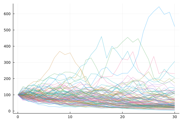
m = BlackScholesMerton(0.01,0.02,.15,100.)

s = ScenarioGenerator(
               1,  # timestep
               30, # projection horizon
               m,  # model
           )

Instantiate an array of the projection with collect(s).

Plotted BSM Example

Plot 100 paths:

using Plots
projections = [collect(s) for _ in 1:100]

p = plot()

for p in projections
    plot!(0:30,p,label="",alpha=0.5)
end

p

Correlated Scenarios

Combined with using Copulas, you can create correlated scenarios with a given copula. See ?Correlated for the docstring on creating a correlated set of scenario generators.

Example

Create two equity paths that are 90% correlated:

using EconomicScenarioGenerators, Copulas

m = BlackScholesMerton(0.01,0.02,.15,100.)
s = ScenarioGenerator(
                      1,  # timestep
                      30, # projection horizon
                      m,  # model
                  )

ss = [s,s] # these don't have to be the exact same, but do need same shape
g = ClaytonCopula(2,7) # highly dependendant model
c = Correlated(ss,g)

x = collect(c) # an array of tuples

using Plots

# get the 1st/2nd value from the scenario points
plot(getindex.(x,1))
plot!(getindex.(x,2))

Other ESG packages

• Python
  • https://github.com/jason-ash/pyesg