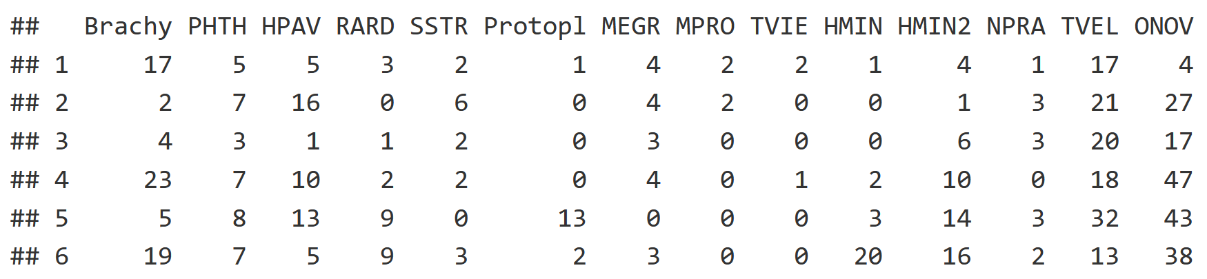
Let's view the dataset! We are working with the mite dataset from Borcard et al. (1992) which contains: community mites data from 70 soil cores, soil core environmental data, and principle components of neighbor matrices.
Starting with the community dataset, each column is a species while each row is a soil core. Each of the mite datasets have 70 rows, with each row being a soil core community.
head(mite[,1:14])
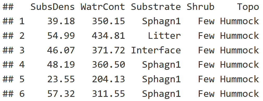
We also have environmental variables for our soil cores, which is further described by the table below.
| Code | Description of variable |
|---|---|
| SubsDens | Substrate density (dry matter) [g dm^-3^] |
| WatrCont | Water content [g dm^-3^] |
| Substrate | Substrate [7 unordered classes; 6 substrate types + interface category] |
| Shrub | Shrubs [3 ordered classes] |
| Topo | Microtopography [Blanket - Hummock] |
head(mite.env)
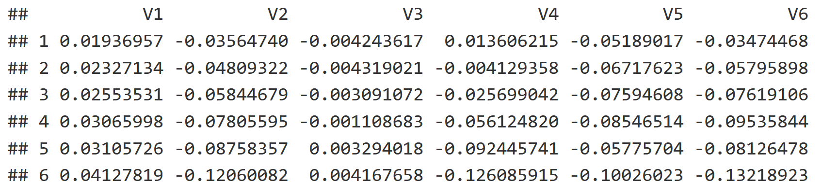
Additionally we have a spatial component in the form of a Principle Component Analysis, which reflects the spatial autocorrelation between soil cores to visualize how different sites are spatially related. The PCNM creates a list of vectors, with each explaining spatial autocorrelation from broader to finer scales (V1 = broad, V5 is finer, V15 is even finer etc.). The last few vectors in the list are essentially interpreting statistical noise. Here is a snapshot of the table, although the scale goes all the way down to V22!
head(mite.pcnm[,1:6])
Background
- Variable Reduction Approach: Unconstrained or indirect ordination method, meaning that you have a single data matrix that you're creating linear combinations of the data to come up with a reduction in the number of variables.
- RDA = Redundancy Analysis: A form of constrained or direct ordination where we have two matrices, usually a community matrix and an environmental matrix. Aims to describe how much variation in the community matrix can we explain given the environmental data.
- If the rda() function from the vegan package is given a single matrix, it will run a Principle Component Analysis (PCA)!
# 1. Run the Principle Component Analysis (PCA)
PCA = rda(mite.env[1:2])
# 2. View PCA
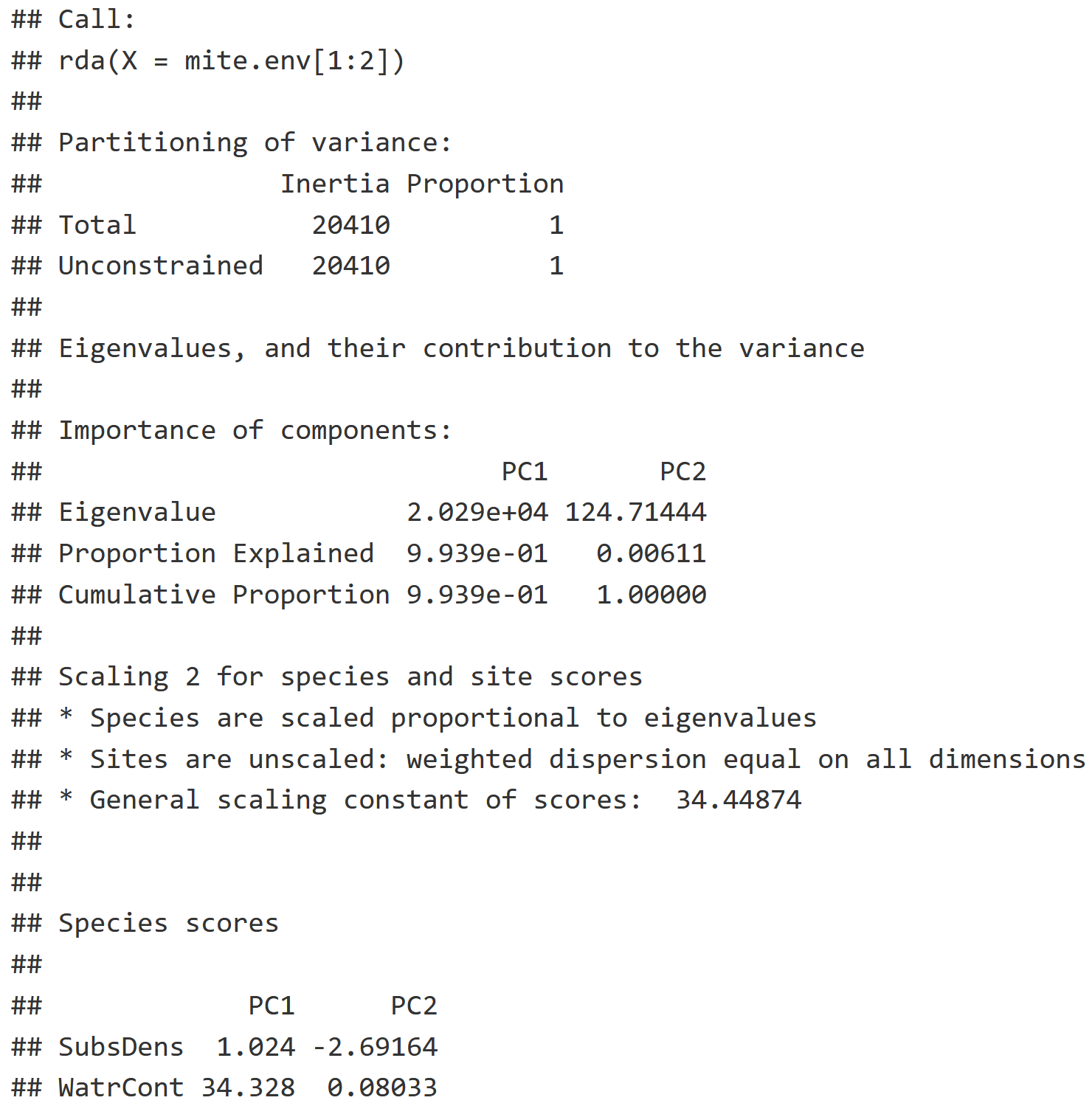
summary(PCA)
PCA Interpretation
- Inertia: How much variance can we explain with environmental data, relating to the concept of 'constrained ordination'.
- Note: If you are running a PCA like we are here, their variances remain unconstrained as reflected by identical inertia values in "Total" & "Unconstrained".
- We are creating a Principle Component, or a linear combination, where most of that variation should be explained in the first axis (PC1), and the next most amount of variation is explained by the next axis (PC2) etc. with more exis for each layer of environmental data you use.
- Proportion: Of the variation that is explained, notice 99.39% of the variation in the relationship between our two variables (PC1 & PC2) is explained by PC1.
- Species Scores: This naming is misleading because we are talking about environmental variables, but it tells us where substrate density and water content fall out along PC1 and PC2.
# 3. Plot PCA
autoplot(PCA, arrows=TRUE)
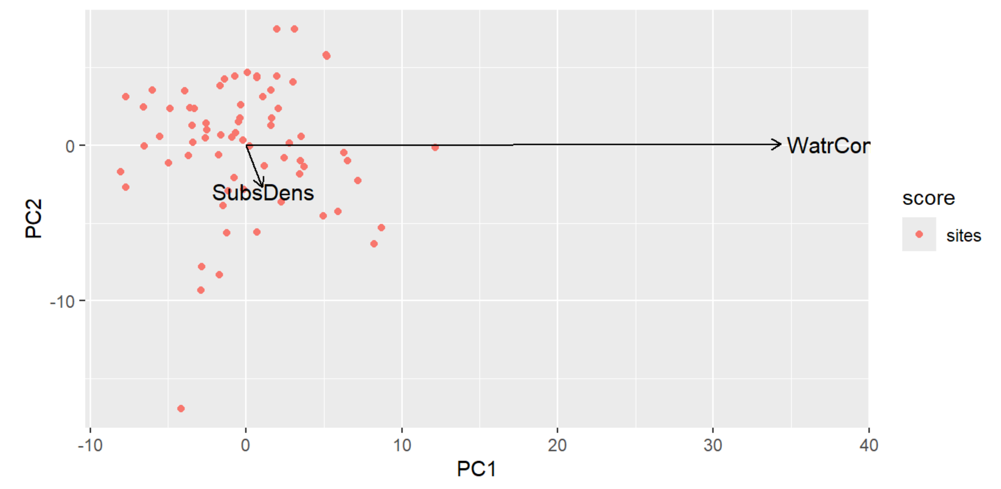
PCA Plot Interpretation
- We have essentially collapsed our two environmental variables into a single axis (the vector), hence the term 'variable reduction' mentioned earlier.
- PC1 (SubsrateDensity) has a short vector along the the PC2 (WaterContent) axis, representing that there's a weak influence by PC2 on PC1.
- PC2 (WaterContent) has a very long vector that's going along PC1 axis, representing that there's a strong influence by PC1 on PC2.
- The length of the vector indicates how important the variable of that axis is, so because the PC1 vector is short along the PC2 axis, we can conclude it is relatively unimportant.
- Note: The multivariate nature of PCA somewhat compromises what the output numbers actually mean.
# 1. Run the Redundancy Analysis (RDA)
RDA = rda(mite ~ SubsDens + WatrCont, data = mite.env)

# 2. View RDA
RDA
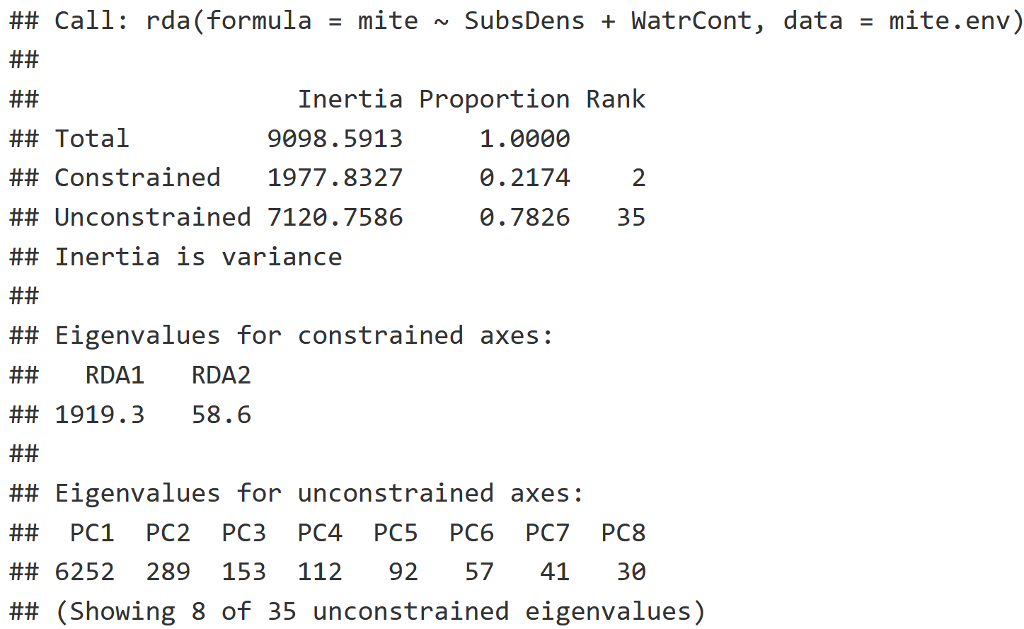
RDA Interpretation
- Constrained Inertia: Amount of variation explained by the environmental variables.
- Unconstrained Inertia: Amount of variation not explained by the environmental variables.
- Proportion: The proportion of variation explained by the constrained and unconstrained inertia respectively.
- It looks like 21.74% of the variation was explained by the environmental variables, and 78.26% of the variation was not explained by the environmental variables.
- Eigenvalues for the Constrained Axis: This is a measure of how much variation is explained by the first axis (RDA1) versus the second axis (RDA2).
- Most of the variation is captured by RDA1 with an eigenvalue of 1919.3 while RDA2 captured much less with an eigenvalue of only 58.6.
# 3. Plot RDA
autoplot(RDA, arrows = TRUE)
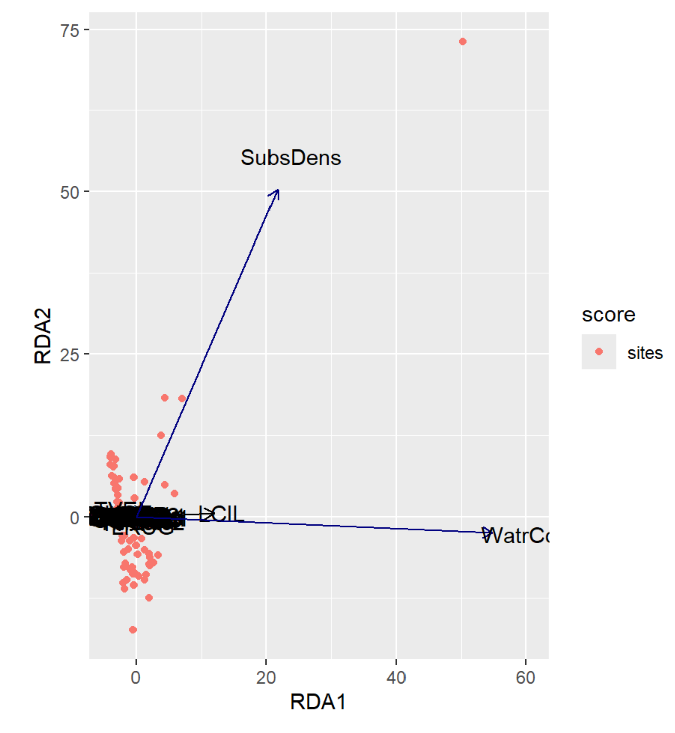
RDA Plot Interpretation
- RDA1 (WaterCont): Positive Score = Sites w/ High Water Content | Negative Score = Sites w/ Low Water Content
- RDA2 (SubDens): Positive Score = Sites w/ High Shrub Density | Negative Score = Sites w/ Low Shrub Density
- Notice how the labels have shifted from PCA1 & PCA2 from the previous unconstrained analysis to RDA1 & RDA2 in the constrained analysis!
- We may want to remove the outlier for a better resolution.
# 1. Run the RDA with more than one Predictor Variable Matrix
RDA_v2 = rda(mite ~ . + as.matrix(mite.pcnm[,1:3]), data = mite.env)

# 2. View RDA
RDA_v2
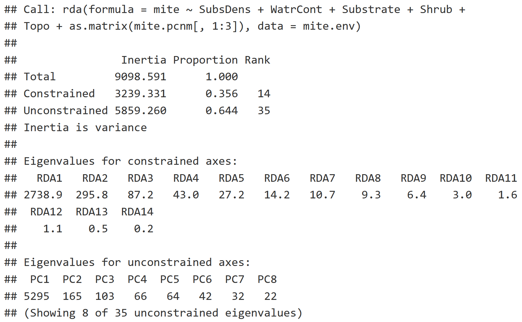
Model Information
- Note the period, which represents that we are using all of the variables from mite.env
- We are only interested in the first three columns of mite.pcnm as we do not need spatial autocorrelation information beyond that degree of resolution. Remember that each proceeding column in the mite.pcnm represents spatial autocorrelation at a finer resolution than the last.
RDA Interpretation
- This model looks to describe how much variation in community composition of mites is explained by environmental variables, and now also spatial autocorrelation data (mite.pcnm).
- The Constrained Inertia, or the variation explained by the environmental variables, has increased from the previous model (21.74%) to 35.6%.
- Notice that we have many more Eigenvalues for all the new environmental variables we've added!
Interpretation Caveats to Consider
- Eigenvalues appear to taper off from RDA3 - RDA14, which poses some difficulty in interpretation: the higher dimension variables may contain information that we are missing, or they are statistical noise.
- We typically want to stick to the first two variables, and sometimes the third or fourth depending on how fast the eigenvalues attenuate from RDA2 onward.
- A solution to this issue is to utilize non-metric multidimensional scaling (NMDS) as a way of showing patterns in only two dimensions.
# 3. Plot RDA
autoplot(RDA_v2, arrows = TRUE)
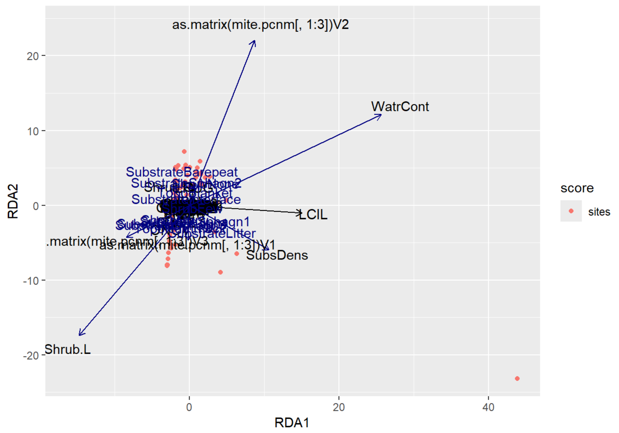
RDA Plot Interpretation
- RDA1 (WaterCont): Positive Score = Sites w/ High Water Content | Negative Score = Sites w/ Low Water Content
- RDA2 (SubDens): Positive Score = Sites w/ High Shrub Density | Negative Score = Sites w/ Low Shrub Density
- There are many sites clustered along the RDA2, indicating that there may be some spatial autocorrelation occurring in the shrub density variable.
The Question: Is there a relative contribution of space versus physical habitat?
# 1. Run the RDA with Two-Group Partitions for Variation Among Space & Environment
v.part = varpart(mite, mite.env[,1:2], mite.pcnm[,1:3])

# 2. View RDA
v.part
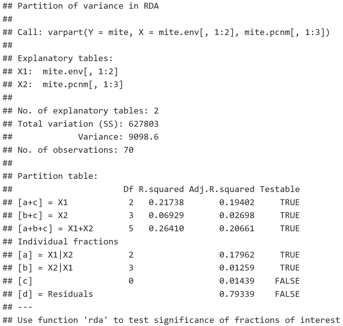
Two-Group Partition RDA Interpretation
- Individual Fractions: Describes what proportion of the variation is explained by each explanatory variable table.
- X1 | X2 : The pure effect of environment while we control for space, which indicates that 17.962% of the variation in the community can be explained with just environmental variables.
- X2 | X1 : The pure effect of the space while we control for the environment, which indicates that 1.259% of the variation in the community can be explained with just the spatial variable.
- [b] Blank : Represents the interaction between X1 & X2, which is 1.439%, and can be visualized in the Venn Diagram plot of v.part below.
# 3. Plot the RDA
plot(v.part)
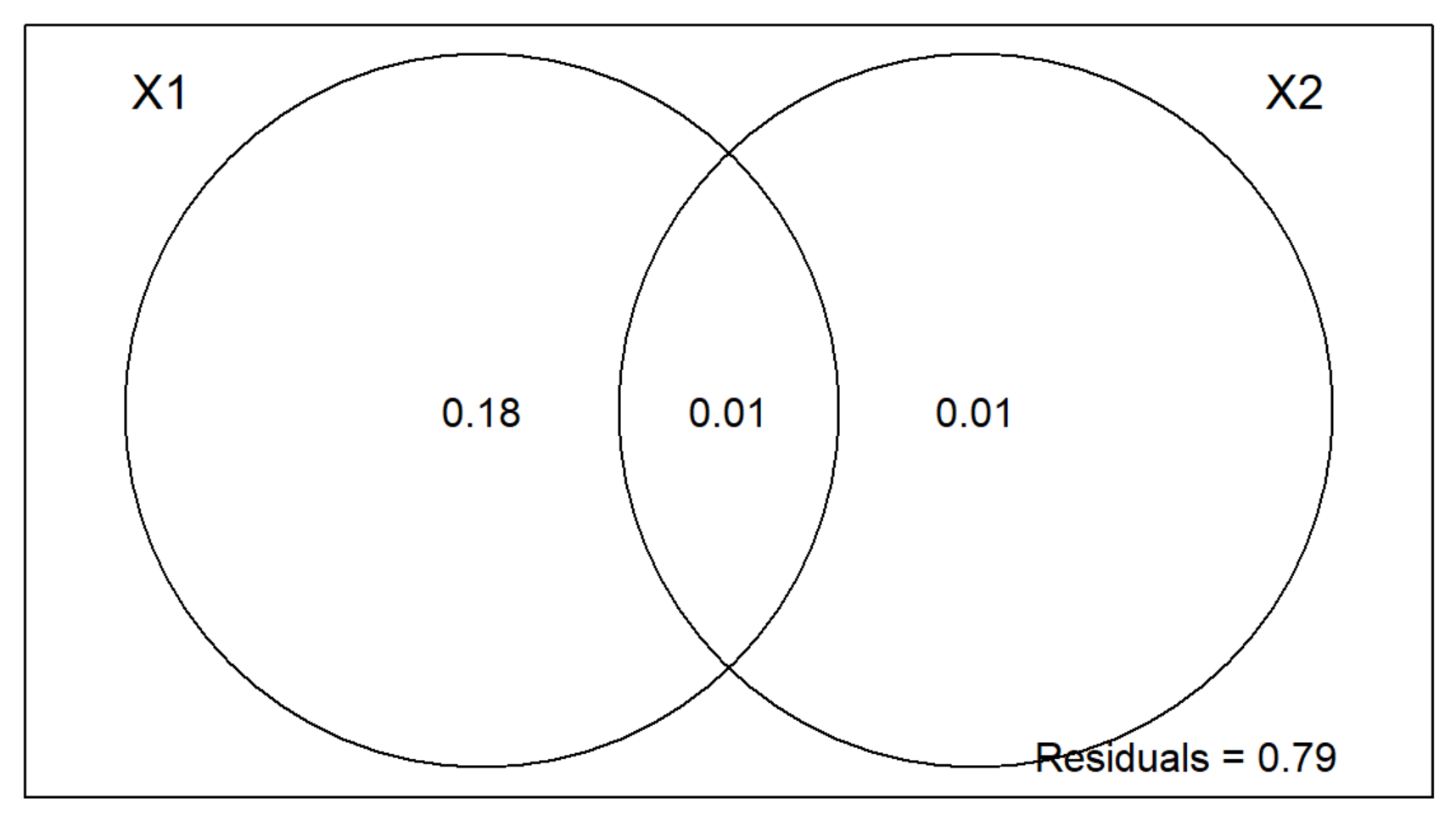
Two-Group Partition RDA Plot Interpretation
- The area outside of the Venn Diagram is the variation (residual error) not accounted for by X1 or X2.
- We can conclude that the environment is much more important than spatial structure for regulating these mite communities.
# 1. Run the RDA with Multi-Group Partitions for Variation Among Space & Environment
v.part.mg = varpart(mite, ~ SubsDens + WatrCont, ~ Substrate +
                      Shrub + Topo, mite.pcnm[,1:3], data = mite.env,
                    transfo = 'hel')

# 2. View RDA
v.part.mg
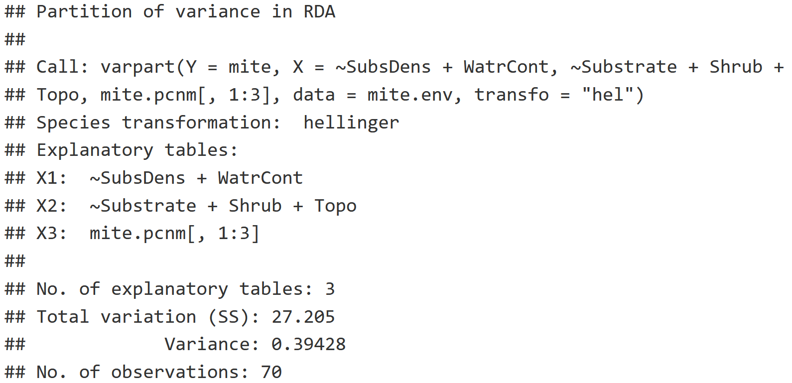
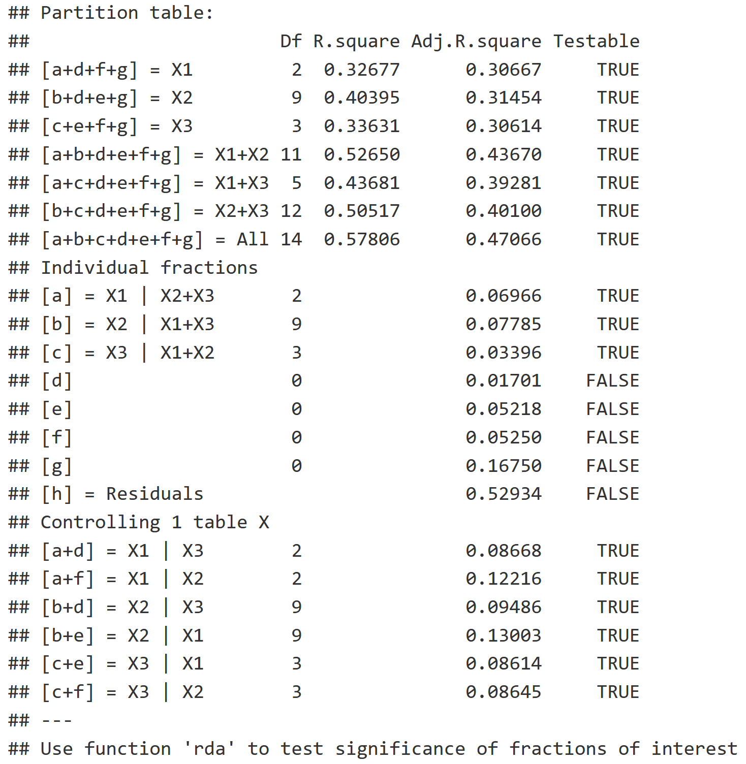
Multi-Group Partition Model Information
- "transfo = 'hel'" : Utilizes the Hellinger transformation to adjust the community data, and down-weight effect of abundant taxa on our ordination. This transformation is commonly used in ecology when you have abundance data.
# 3. Plot the Multi-Group RDA
plot(v.part.mg)
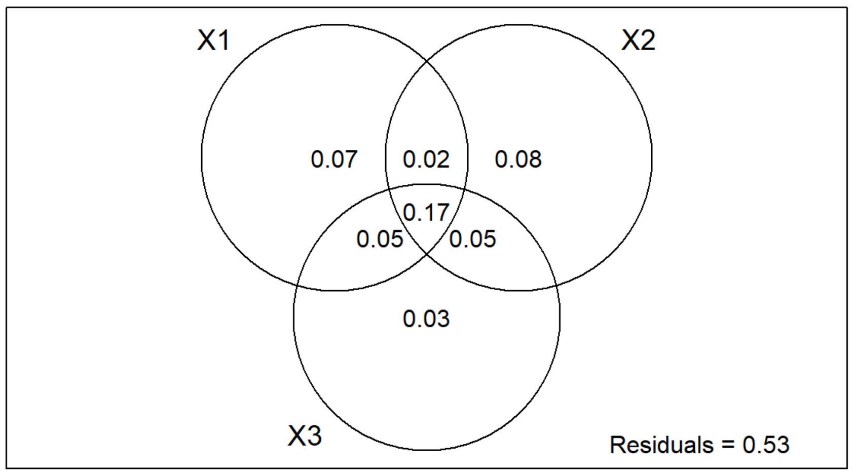
Notice that there are three circles in the Multi-Group Venn Diagram instead of two like in the Two-Group Partition!
Individual Interpretation
- X1 = Continuous Environmental Variables, which explains 7% of the variation.
- X2 = Categorical Environmental Variables, which explains 8% of the variation.
- X3 = Space Variable, which explains 3% of the variation.
Pariwise Interaction Interpretation
- X1 | X2 = 2% of the variation
- X1 | X3 = 5% of the variation
- X2 | X3 = 5% of the variation
- X1 | X2 | X3 = 17% of the variation
Variation Partitioning is a common way to determine the relative contributions/influence of different classes of environmental or spatial predictor variables on community.
The goal of NMDS is to be able to show variation in as few dimensions as possible, so we avoid the issue seen where eigenvalues taper off from RDA3 onward, which poses some difficulty in interpretation.
NMDS accomplishes this by starting with a scatter plot of the data that is based on a PCA, but then iteratively shifts the points a little bit at a time and measures how well these points are represented in two-dimensional space. This allows us to visualize all model variation in only two-dimensions, and avoid omitting these higher dimension eigenvectors (RDA2<).
- Based on Bray-Curtis Distance Measures, which states that a value of zero indicates that the community at Point A is the exact same has the exact same species & abundances as community at Point B. As the value increases from zero towards one, we're either having turnover or loss of species (beta Diversity). You can have new species that come to replace others, or you just lose some species.
- k = 2 : Describes the number of dimensions that we want to consider.
- try = 20 : Number of iterations that we're going to try to show variation in two dimensions, which is by default 20 times.
- Note that upon running metaMDS() it automatically transforms your data by default to a Square Root Transform, and uses a Wisconsin double standardization. You want this because if you're using raw abundance data, it accounts for the issue of abundant taxa having an undue influence on location.
# 1. Create Non-Metric Multidimensional Scaling for Mites
NMDS = metaMDS(mite)

# 2. Plot NMDS
autoplot(NMDS, geom = "text", legend = "none")
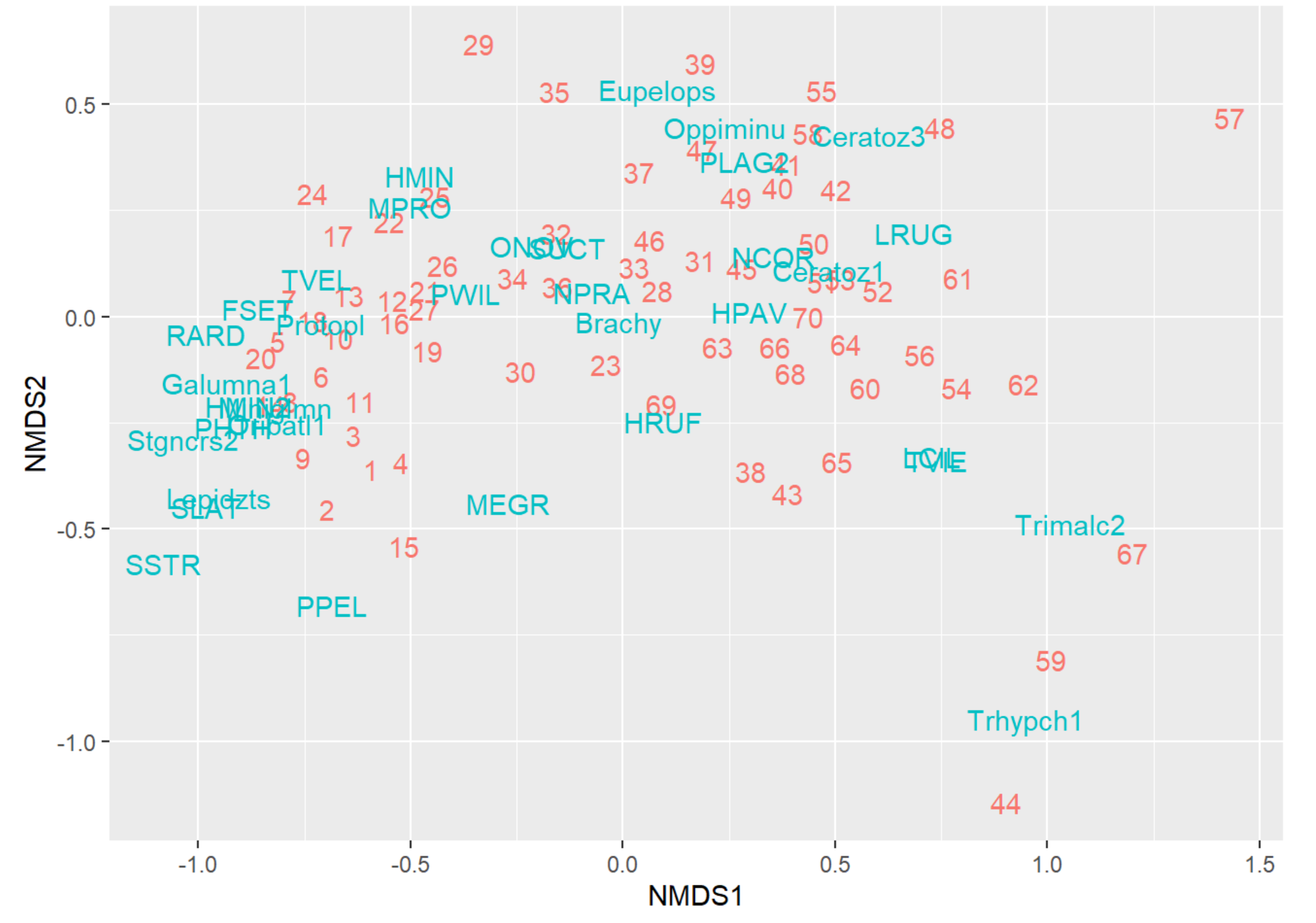
NMDS Model Interpretation
- If your Two-Dimensional "Stress" is <0.2, you are ok to interpret the graphic-but we are really aiming for <.15 or <.1 which is where we start to build a lot of confidence that our Two-Dimensional representation of the data is as good as a Three-Dimensional representation.
- If our 2D "Stress" is 0.2<, we may want to consider modifying (k = 2) to (k = 3) to interpret in Three-Dimensions.
- We get the feedback "No convergence" which indicates that metaMDS() did not find the solution to minimize the stress. You may want to consider increasing the default (try = 20) parameter above 20 iterations.
NMDS Plot Interpretation
- NMDS1: Score = Community # Contains Higher Abundances of the associated Taxa in those Communities
The adonis() function from vegan allows us to create a permuted multi-variate analysis of variance, and looks to predict your response variable (mites) based off a categorical variable (Shrubs).
- Again we are using the Bray-Curtis Distances!
# 1. Test for Differences in Communities Among Shrub Groups (
# Shrub Groups: None, Few, Many
shrub.com = adonis2(mite ~ Shrub,
                   data = mite.env,
                   permutations = 999,
                   method = "bray")

# 2. View Adonis Output
shrub.com
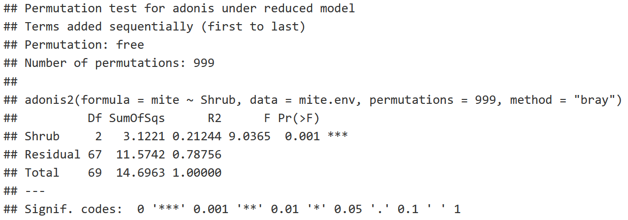
Statistics Background
- The larger the F Model (F Statistic), the more likely you're going to have a significant relationship between variables.
- P-value: The probability that we're going to find an F Statistic equal to or greater than 9.0365.
Adonis Interpretation
- P-value is <0.05, indicating that there is a statistically signficant difference between the Shrub Groups (None, Few, Many).
- R2: 21.244% of the variation in the community structure is explained by the shrub factor, with the remaining 78.756% being unexplained as residuals.
Conclusion: There is a significant difference in mite community structure among sites with None, Few, and Many Shrubs!
- Note that we assume that variance is equal among the shrub groups to make this conclusion!
# 1. Create Pairwise Distances between All Locations
mite.dist = vegdist(mite)

# 2. Determine Differences in Dispersion of the data
#    within our Distance Classes based on Shrub Group
mite.bdesp      = betadisper(mite.dist, mite.env$Shrub)
mite.dist.anova = anova(mite.bdesp)

# 3. View ANOVA
mite.dist.anova
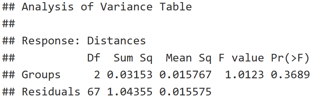
Interpretation
- F-value is low and P-value is high, indicating that the variance within these Shrub groups (None, Few, Many) is equal.
- This indicates that the adonis2() test above is valid!
# 1. Create Continuous NMDS Model Test
mite.cont = envfit(NMDS ~ SubsDens + WatrCont, mite.env)

# 2. View Model
mite.cont
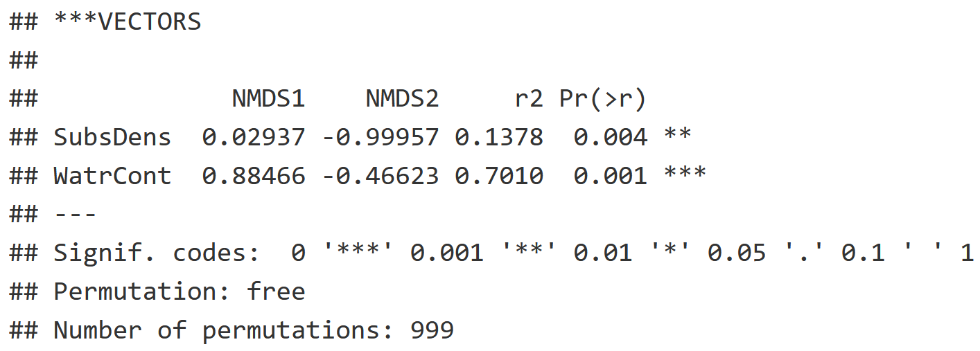
Interpretation
- P-values for both SubsDens & WatrCont are <0.05, indicating that there is a significant test of relationship between the environmental variables in the community structure.
- R2 indicates that 13.81% of the variation in the mite community can be explained by substrate density measure, and 70.09% of the variation in the mite community can be explained by water content.
We can conclude that there is variation in the community structure of mites across the seven samples in the landscape, and that it is related to shrub density classes (None, Few, Many), and they are distributed across the landscape along a gradient of water content.