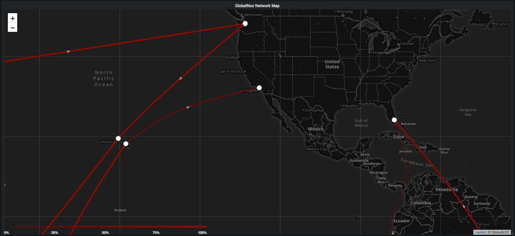
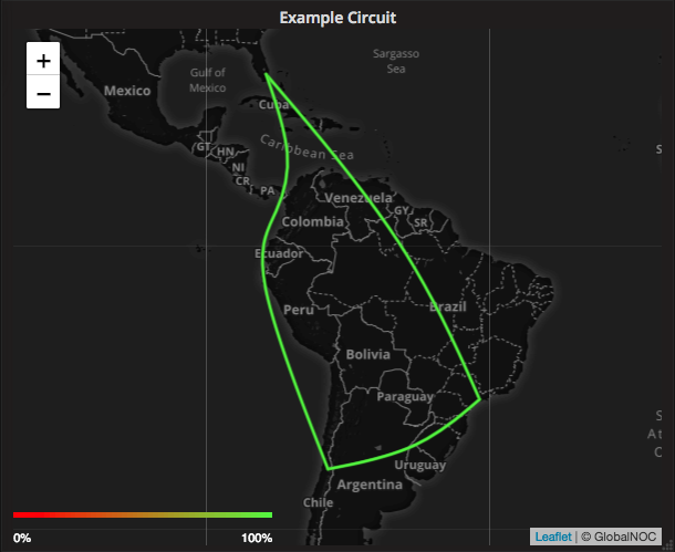
The Network Map Panel is a world map that provides the ability to monitor and visualize realtime traffic statistics. It uses timeseries data to represent traffic between nodes as circuits. It provides this information when hovered over the circuits and nodes.
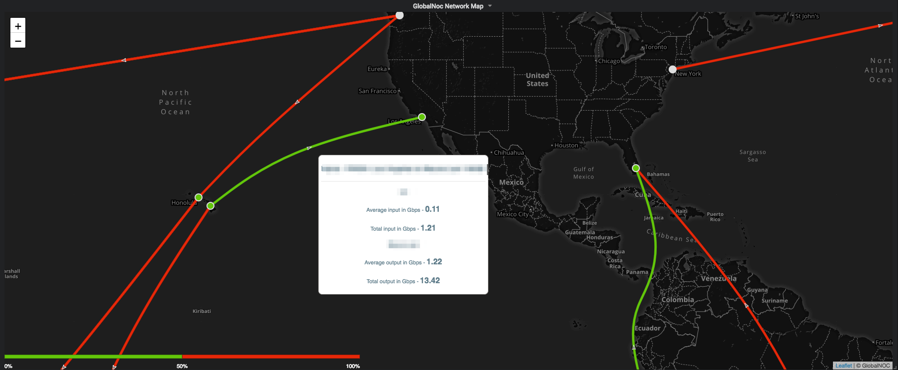
The Network Map Panel also provides the ability to configure different map options and display options.
-
Map Options

-
Map URL: A valid map url should be provided so that the map loads with all the tiles. In the screenshot below, mapbox api is used to specify the map tiles. A valid access token is necessary for the mapbox API.
-
Hide Layers with no values: This option allows the user to hide any layers/circuits when there's no data returned for them.
-
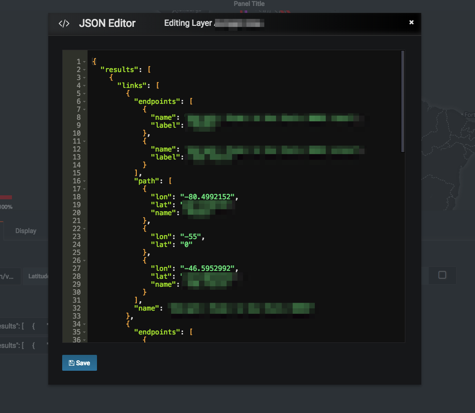
JSON Editor: Double clicking the 'Map Source' label or its input field opens a JSON Editor modal. This editor makes use of grafana's code-editor directive to provide the user with code editor capabilities such as syntax highlighting, error detection, collapsible fields etc.
-
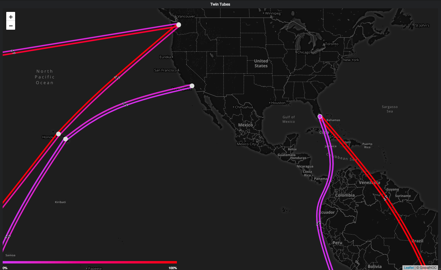
Twin Tubes: Checking this option switches the adjacency links on the map to twin tubes mode. Each line has a directional arrow associated with it.
-
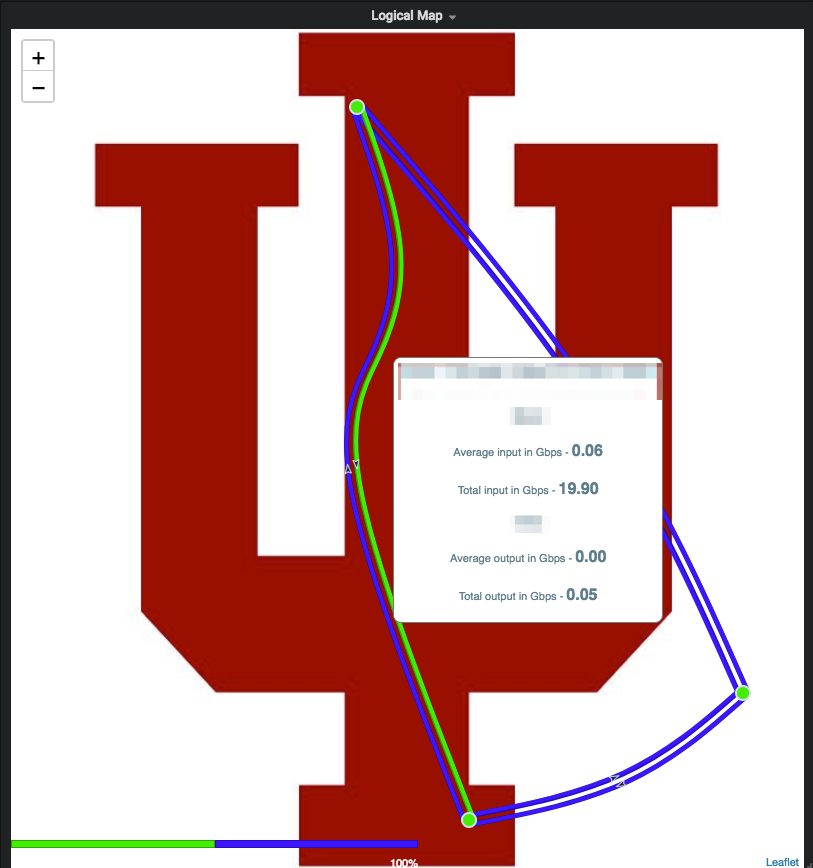
Logical Map: Checking the Use Image option allows the user to make use of logical maps. The image below shows the options available to create a logical map.
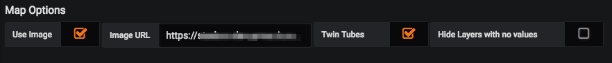
- Image URL: A valid url to an image should be provided to create a logical map with that image.
-
-
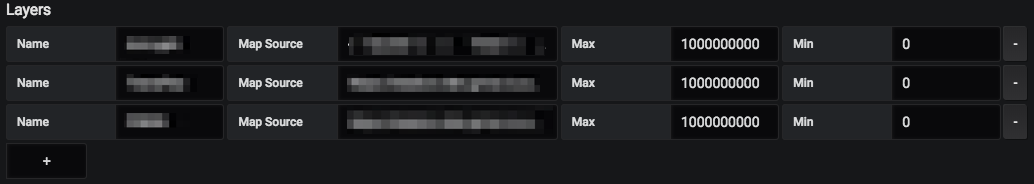
Layers: Different layers/circuits can be added to the map using this option. A valid Map Source is required to add each layer on to the map.
Example map source json object.
{
  "results": [
    {
      "links": [
        {
          "endpoints": [
	    {
	      "name": "enpoint1 to endpoint2 input",
              "label": "label for endpoint1"
	    },
	    {
	      "name": "endpoint1 to endpoint2 output",
              "label": "label for endpoint2"
	    }
	  ],
          "path": [
            {
              "lon": "138.8671875",
              "order": "10",
              "lat": "36.0313317763319"
            },
            {
              "lon": "-122.335927373024",
              "order": "20",
              "lat": "47.5652166492485"
            }
          ],
          "name": "Link Name"
        }
      ],
      "endpoints": [
        {
          "pop_id": null,
          "lon": "139.853142695116",
          "real_lon": null,
          "real_lat": null,
          "name": "endpoint1",
          "lat": "35.7653023546885"
        },
        {
          "pop_id": null,
          "lon": "-122.335927373024",
          "real_lon": null,
          "real_lat": null,
          "name": "endpoint2",
          "lat": "47.5652166492485"
        }
      ]
    }
  ]
}
- Ability to set the map's center by providing the lat and long coordinates.
- Ability to specify the zoom level on the map.
Display tab provides different options for the user to customize the monitoring experience of the metrics on the map.
-
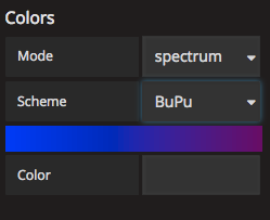
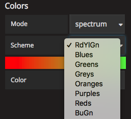
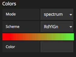
Colors: Ability to change the color scheme for the layers on the map based on two different modes.
- Mode: Spectrum. This mode currently has 19 different color schemes to choose from.
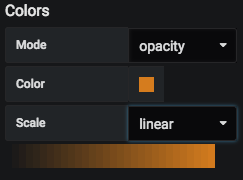
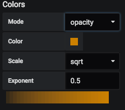
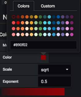
- Mode: Opacity. This mode provides the ability to choose from two different scales, i.e., linear, sqrt. It also provides the option to choose a custom color from the color picker.
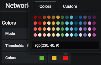
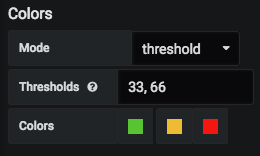
- Mode: Threshold. This mode provides the ability to specify thresholds as comma separated values between 0 and 100 i.e. 0 < thresholds < 100. It provides the ability to choose a distinct color for each threshold.
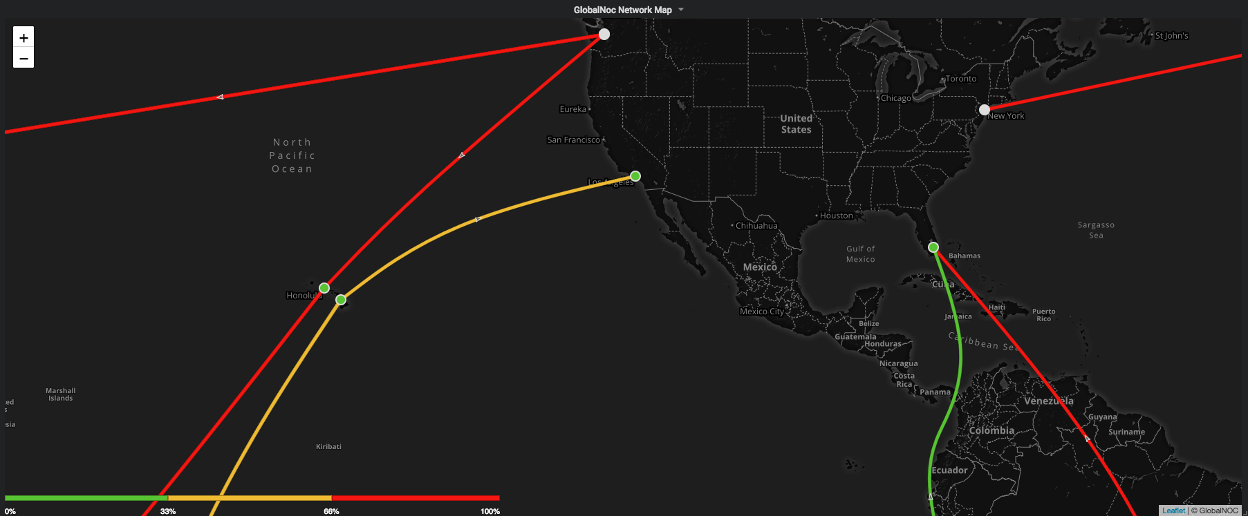
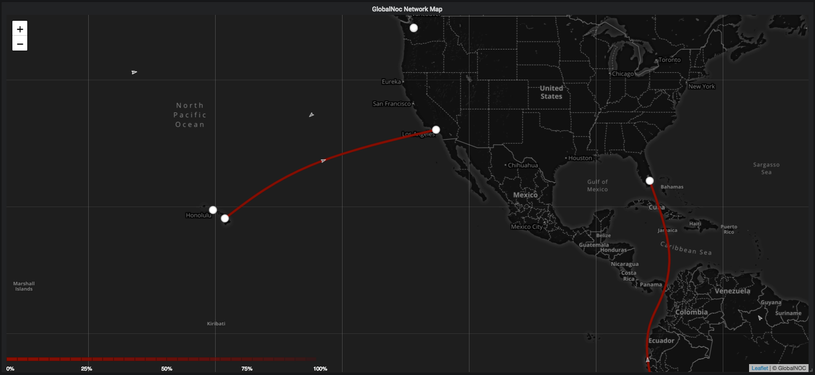
- Legend: Invert legend. This option inverts the current legend on the map and also affects the map to use the inverted scheme.
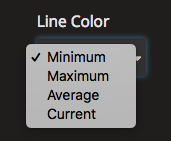
- Line Color: Ability to choose the behavior of the line colors based on metric.
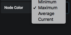
- Node Color: Ability to choose the behavior of the node colors based on metric.
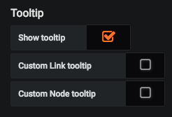
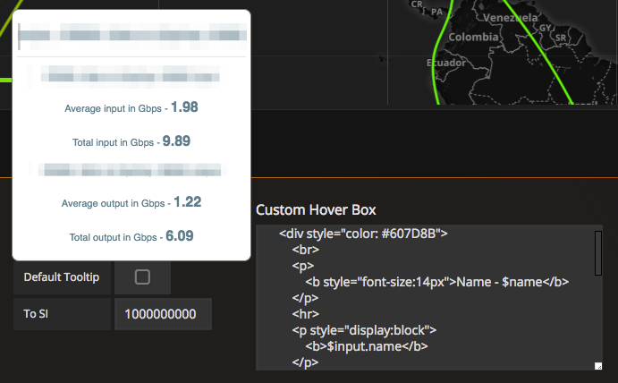
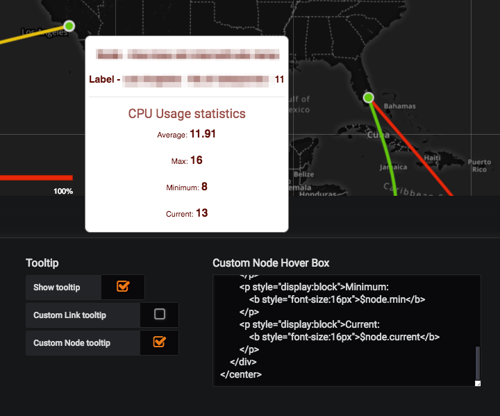
- Tooltip: Ability to customize the tooltip for the map. It also provides an option for the user to enter html to have a customized link hover box and customized node hover box.
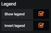
- Show or Hide Legend
- Show or Hide Tooltip
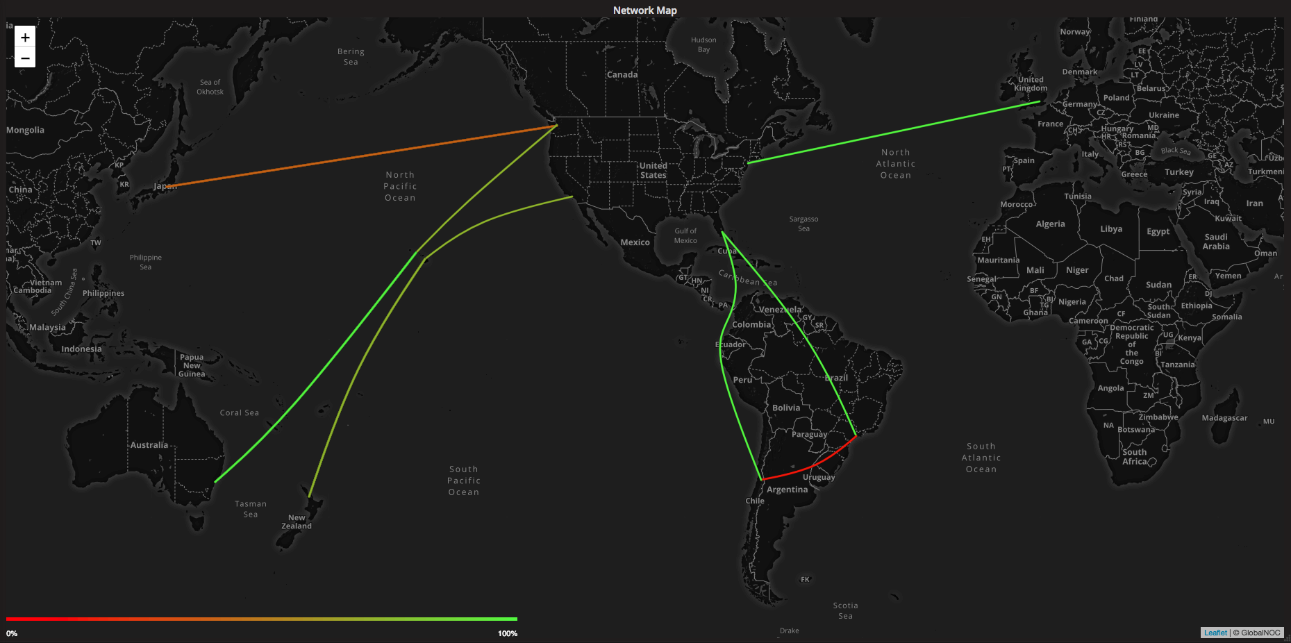
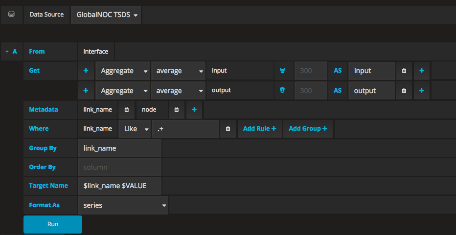
The Network Map Panel takes the timeseries data to represent the traffic between nodes. An example of a query is as follows. Note that the query is for the GlobalNoc's TSDS Datasource.
get link_name, node, aggregate(values.input, 60, average), aggregate(values.output, 60, average) between (1520024588, 1520024888) by link_name from interface where (link_name like ".+")
The query can also be built using the visual query builder from the metrics tab in the map editor. It is shown in the picture below.
Example of the response dataList that is used by the Network Map Panel to process and render the circuits is shown in the block below.
{
  "dataList": [
  {
     "datapoints": [
        [32583665.47, 1520260620000],[28523481.33, 1520260680000],[23701115.87, 1520260740000],[26656626.8, 1520260800000],[null, 1520260860000]
     ],
     "name": "aggregate(values.input, 60, average)",
     "target": "endpoint1 to endpoint2 input"
  },
  {
     "datapoints": [
      [1171793116.67, 1520260620000],[1075541011.2, 1520260680000],[1005332018.67, 1520260740000],[1087891948.67, 1520260800000],[null, 1520260860000]
     ],
     "name": "aggregate(values.output, 60, average)",
     "target": "endpoint1 to endpoint2 output"
  },
  {...},
  {...}
  ]
}
The target name from each data object in the dataList is matched with the endpoints from the map source json object provided by the user. This allows the map to show the appropriate information for each circuit returned by the TSDS query.
This section demonstrates how the map topology is lined up with the data returned by the TSDS query.
{
    "dataList":[
        {
            "name": "aggregate(values.input, 60, average)", "target": "A: endpoint2 to endpoint3 input", "datapoints": [[32583665.47, 1520260620000],[...],[...]]
        },
        {
            "name": "aggregate(values.output, 60, average)", "target": "A: endpoint2 to endpoint3 output", "datapoints": [[...],[...],[...]]
        },
        {
            "name": "aggregate(values.input, 60, average)", "target": "A: endpoint1 to endpoint2 input", "datapoints":[[...],[...],[...]]
        },
        {
            "name": "aggregate(values.output, 60, average)", "target": "A: endpoint1 to endpoint2 output", "datapoints": [[...],[...],[...]]
        },
        {
            "name": "aggregate(values.input, 60, average)", "target": "A: endpoint1 to endpoint3 input", "datapoints": [[...],[...],[...]]
        },
        {
            "name": "aggregate(values.output, 60, average)", "target": "A: endpoint1 to endpoint3 input", "datapoints": [[...],[...],[...]]
        },
        {
            "name": "aggregate(values.input, 60, average)", "target": "B: endpoint1 to endpoint2 input", "datapoints": [[...],[...],[...]]
        },
        {
            "name": "aggregate(values.output, 60, average)", "target": "B: endpoint1 to endpoint2 output", "datapoints": [[...],[...],[...]]
        },
        {
            "name": "aggregate(values.input, 60, average)", "target": "C: endpoint2 to endpoint3 input", "datapoints": [[...],[...],[...]]
        },
        {
            "name": "aggregate(values.output, 60, average)", "target": "C: endpoint2 to endpoint3 output", "datapoints": [[...],[...],[...]]
        },
        {
            "name": "aggregate(values.input, 60, average)", "target": "C: endpoint3 to endpoint4 input", "datapoints": [[...],[...],[...]]
        },
        {
            "name": "aggregate(values.output, 60, average)", "target": "C: endpoint3 to endpoint4 output", "datapoints": [[...],[...],[...]]
        },
        {
            "name": "aggregate(values.input, 60, average)", "target": "C: endpoint5 to endpoint4 input", "datapoints": [[...],[...],[...]]
        },
        {
            "name": "aggregate(values.output, 60, average)", "target": "C: endpoint5 to endpoint4 output", "datapoints": [[...],[...],[...]]
        },
        {
            "name": "aggregate(values.input, 60, average)", "target": "C: endpoint1 to endpoint5 input", "datapoints": [[...],[...],[...]]
        },
        {
            "name": "aggregate(values.output, 60, average)", "target": "C: endpoint1 to endpoint5 output", "datapoints": [[...],[...],[...]]
        },
        {
            "name": "aggregate(values.input, 60, average)", "target": "D: endpoint1 to endpoint2 input", "datapoints": [[...],[...],[...]]
        },
        {
            "name": "aggregate(values.output, 60, average)", "target": "D: endpoint1 to endpoint2 output", "datapoints": [[...],[...],[...]]
        }
    ]
}
The target names from the above dataList are matched with the endpoints from links field in the Map Source JSON object.
{
  "results": [
    {
      "links": [
        {
          "endpoints": [
	     {
	       "name": "A: endpoint1 to endpoint3 input",
	       "label": "label for endpoint"
	     },
	     {
	       "name": "A: endpoint1 to endpoint3 output",
	       "label": "label for endpoint"
	     }
          ],
          "path": [
            {
              "lon": "-80.4992152",
              "lat": "26.2118715",
              "name": "ep1"
            },
            {
              "lon": "-55",
              "lat": "0"
            },
            {
              "lon": "-46.5952992",
              "lat": "-23.6824124",
              "name": "ep3"
            }
          ],
          "name": "A: endpoint1 to endpoint3"
        },
        {
          "endpoints": [
	    {
	      "name": "A: endpoint2 to endpoint3 input",
	      "label": "label for endpoint"
	    },
	    {
	      "name": "A: endpoint2 to endpoint3 output",
	      "label": "label for endpoint"
	    }
          ],
          "path": [
            {
              "lon": "-46.5952992",
              "lat": "-23.6824124",
              "name": "ep3"
            },
            {
              "lon": "-55",
              "lat": "-32"
            },
            {
              "lon": "-70.6791936",
              "lat": "-33.4533673",
              "name": "ep2"
            }
          ],
          "name": "A: endpoint2 to endpoint3"
        },
        {
          "endpoints": [
	    {
	      "name": "A: endpoint1 to endpoint2 input",
	      "label": "label for endpoint"
	    },
	    {
	      "name": "A: endpoint1 to endpoint2 output",
	      "label": "label for endpoint"
	    }
          ],
          "path": [
            {
              "lon": "-70.6791936",
              "lat": "-33.4533673",
              "name": "ep2"
            },
            {
              "lon": "-88",
              "lat": "5"
            },
            {
              "lon": "-79.7240525",
              "lat": "9.1422762"
            },
            {
              "lon": "-75",
              "lat": "15"
            },
            {
              "lon": "-80.4992152",
              "lat": "26.2118715",
              "name": "ep1"
            }
          ],
          "name": "A: endpoint1 to endpoint2"
        }
      ],
      "endpoints": [
        {
          "lon": "-80.4992152",
          "lat": "26.2118715",
          "name": "endpoint1 cpu",
	  "label": "endpoint1 label"
        },
        {
          "lon": "-46.5952992",
          "lat": "-23.6824124",
          "name": "endpoint2 cpu",
	  "label": "endpoint2 label"
        },
        {
          "lon": "-70.6791936",
          "lat": "-33.4533673",
          "name": "endpoint3 cpu",
	  "label": "endpoint3 label"
        }
      ]
    }
  ]
}
Network Map converts the map source json into an array of links and endpoints. Each element in the links array is an object that is represented in the block below.
[
  {
	  "endpoints": [{"name": "A: endpoint1 to endpoint3 input", "label": "label for endpoint"},{"name": "A: endpoint1 to endpoint3 output", "label": "label for endpoint"}].
	  "link_id": "link_1234",
	  "name": "A: endpoint1 to endpoint3",
	  "path": [{lat,lng,name,...},{lat,lng,name,...},{lat,lng,name,...}]
  },
  {...},
  {...},
  {...},
    .
    .
    .
]
The map renders circuits if the endpoints.name of these links match with the target in the dataList array. In addition, the corresponding data for each circuit is used to calculate the metrics to be shown on the map.
In the example above, the first six results in the dataList object match with the endpoints.name from each of the three links. Therefore, the network map renders three circuits for the provided map source json object.
The Network Map Panel makes use of the following libraries:
- Leaflet
- D3
- Lodash