music genre classification : GRU vs Transformer
python -m pip install -r requirements.txt
-
Uncompress the data zips (fma_metadata.zip, fma_large.zip).
-
Run prepare_data.py with the correct paths to genrate mapping files.
-
Run audio_processing.py with the correct paths to genrate .npy files.
-
Run training with rnn_genre_classification.py or trsf_genre_classification.py
-
To predict on new mp3s run predict.py with the correct paths.
The objective of this post is to implement a music genre classification model by comparing two popular architectures for sequence modeling: Recurrent Neural networks and Transformers.
RNNs are popular for all sorts of 1D sequence processing tasks, they re-use the same weights at each time step and pass information from a time-step to the next by keeping an internal state and using a gating mechanism (LSTM, GRUs … ). Since they use recurrence, those models can suffer from vanishing/exploding gradients which can make training and learning long-range patterns harder.
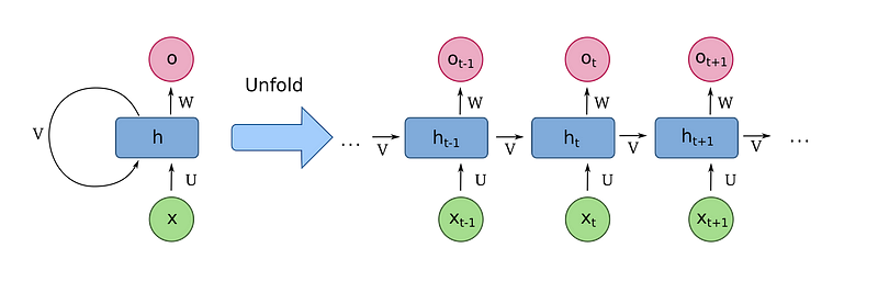
Source: https://en.wikipedia.org/wiki/Recurrent_neural_network by fdeloche Under CC BY-SA 4.0
Transformers are a relatively newer architecture that can process sequences without using any recurrence or convolution [https://arxiv.org/pdf/1706.03762.pdf]. The transformer layer is mostly point-wise feed-forward operations and self-attention. These types of networks are having some great success in natural language processing, especially when pre-trained on a large amount of unlabeled data [https://arxiv.org/pdf/1810.04805].
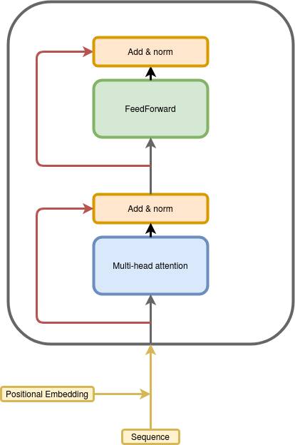
Transformer Layer — Image by author
We will use the Free Music Archive Dataset https://github.com/mdeff/fma/ and more specifically the large version with 106,574 tracks of 30s, 161 unbalanced genres, which sums to a total of 93 Gb of music data. Each track is labeled with a set of genres that best describe it.
"20": [
        "Experimental Pop",
        "Singer-Songwriter"
    ],
    "26": [
        "Experimental Pop",
        "Singer-Songwriter"
    ],
    "30": [
        "Experimental Pop",
        "Singer-Songwriter"
    ],
    "46": [
        "Experimental Pop",
        "Singer-Songwriter"
    ],
    "48": [
        "Experimental Pop",
        "Singer-Songwriter"
    ],
    "134": [
        "Hip-Hop"
    ]
Our target in this project is to predict those tags. Since a song can be attached to more than one tag it can be formulated as a multi-label classification problem with 163 targets, one for each class.
Some classes are very frequent like Electronic music for example where exists for 22% of the data but some other classes appear very few times like Salsa where it contributes by 0.01% of the dataset. This creates an extreme imbalance in the training and evaluation, which leads us to use the micro-average area under the precision-recall curve as our metric.
|     | Genre                    |   Frequency |    Fraction |
|----:|:-------------------------|------------:|------------:|
|   0 | Experimental             |       24912 | 0.233753    |
|   1 | Electronic               |       23866 | 0.223938    |
|   2 | Avant-Garde              |        8693 | 0.0815677   |
|   3 | Rock                     |        8038 | 0.0754218   |
|   4 | Noise                    |        7268 | 0.0681967   |
|   5 | Ambient                  |        7206 | 0.067615    |
|   6 | Experimental Pop         |        7144 | 0.0670332   |
|   7 | Folk                     |        7105 | 0.0666673   |
|   8 | Pop                      |        6362 | 0.0596956   |
|   9 | Electroacoustic          |        6110 | 0.0573311   |
|  10 | Instrumental             |        6055 | 0.056815    |
|  11 | Lo-Fi                    |        6041 | 0.0566836   |
|  12 | Hip-Hop                  |        5922 | 0.055567    |
|  13 | Ambient Electronic       |        5723 | 0.0536998   |
.
.
.
| 147 | North African            |          40 | 0.000375326 |
| 148 | Sound Effects            |          36 | 0.000337793 |
| 149 | Tango                    |          30 | 0.000281495 |
| 150 | Fado                     |          26 | 0.000243962 |
| 151 | Talk Radio               |          26 | 0.000243962 |
| 152 | Symphony                 |          25 | 0.000234579 |
| 153 | Pacific                  |          23 | 0.000215812 |
| 154 | Musical Theater          |          18 | 0.000168897 |
| 155 | South Indian Traditional |          17 | 0.000159514 |
| 156 | Salsa                    |          12 | 0.000112598 |
| 157 | Banter                   |           9 | 8.44484e-05 |
| 158 | Western Swing            |           4 | 3.75326e-05 |
| 159 | N. Indian Traditional    |           4 | 3.75326e-05 |
| 160 | Deep Funk                |           1 | 9.38315e-06 |
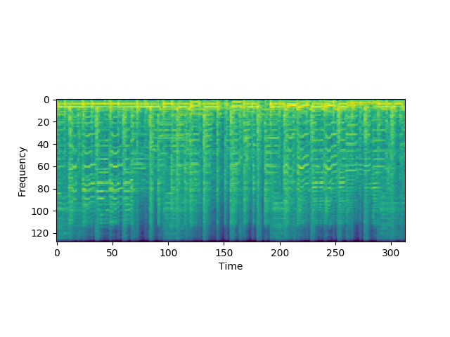
We use Mel-Spectrograms as input to our networks since its a denser representation of the audio input and it fits the transformer architecture better since it turns the raw audio-waves into a sequence of vectors.
def pre_process_audio_mel_t(audio, sample_rate=16000):
        mel_spec = librosa.feature.melspectrogram(y=audio, sr=sample_rate,
                                                  n_mels=n_mels)
        mel_db = (librosa.power_to_db(mel_spec, ref=np.max) + 40) / 40

    mel_db.T
Each 128-D vector on the Time axis is considered an element of the input sequence.
Loading the audio file and sub-sampling it to 16kHz and then computing the Mel-spectrograms can take a significant amount of time, so we pre-compute and save them on disk as a .npy file using NumPy.save.
I choose the hyper-parameters so that both the RNNs and Transformers have a similar number of trainable parameters.
The only difference between the two models is the encoder part being either a transformer or bi-directional GRU. The two models have 700k trainable parameters.
We will evaluate each genre using the area under the precision-recall curve and then micro-average across classes.
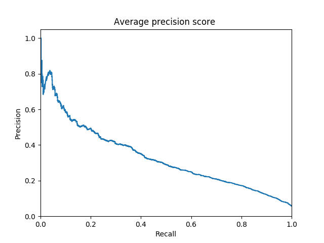
Hip-hop PR Curve for the transformer
RNN vs Transformer AUC PR =>
transformer micro-average     :  0.20
rnn micro-average             :  0.18
We can see that the transformer works a little better than GRU. We can improve the performance by doing some Test-Time augmentation and averaging the prediction of multiple crops of the input sequence.
Test-Time Augmentation =>
transformer micro-average     :  0.22
rnn micro-average             :  0.19
The results overall seem a little weak, it is probably due to the great number of classes that make the task harder or maybe due to the class imbalance. One possible improvement is to ditch the multi-label approach and work on a ranking approach, since its less sensitive to class imbalance and the big number of classes.
Top 5 predictions:
('Folk', 0.7591149806976318)
('Pop', 0.7336021065711975)
('Indie-Rock', 0.6384000778198242)
('Instrumental', 0.5678483843803406)
('Singer-Songwriter', 0.558732271194458)
('Electronic', 0.8624182939529419)
('Experimental', 0.6041183471679688)
('Hip-Hop', 0.369397908449173)
('Glitch', 0.31879115104675293)
('Techno', 0.30013027787208557)
In this post, we compared two popular architectures for sequence modeling RNNs and Transformers. We saw that transformers slightly over-performs GRUs which shows that Transformers can be a viable option to test even outside Natural Language Processing.
TF2 Transformers : https://github.com/tensorflow/docs/blob/master/site/en/tutorials/text/transformer.ipynb