Delta Parallel Robot - Trajectory Planning

---

A word from me: This repository is dedicated to studying the different trajectory planning methods (theory + practical). If you need to ask any questions you can reach me via email or linked-in.

Overview:

• Introduction
• Theoretical Analysis of Trajectory Plannig Methods
  • point-to-point trajectory planning
    • 3-4-5 interpolating polynomial
    • 4-5-6-7 interpolating polynomial
    • Point-to-Point Trapezoidal method
  • multi-point trajectory planning
    • Higher Order Polynomials
    • Cubic-Spline
    • Improved Cubic-Spline
    • Multi-point Trapezoidal
  • Visual Results
• Experimental Implementation
• References

1 - Introduction

---

History

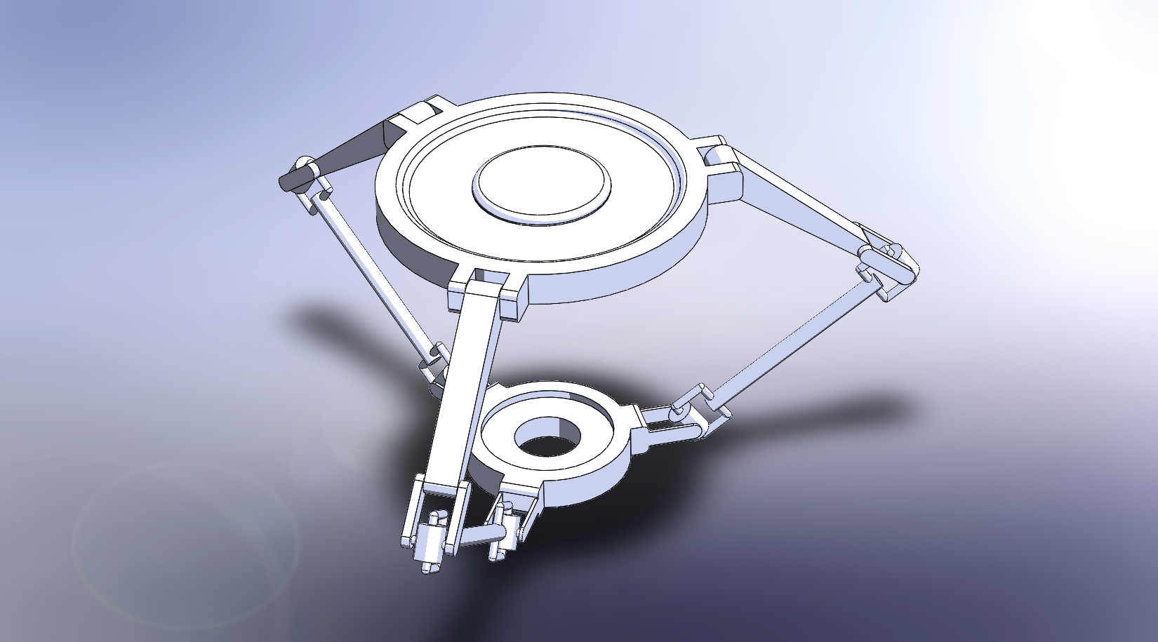
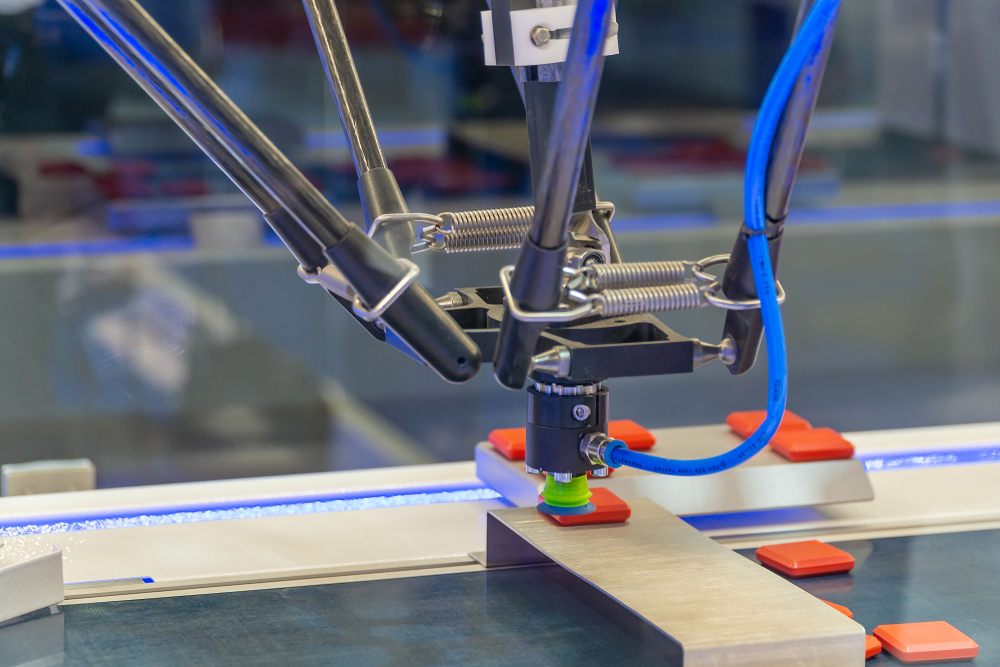
Delta Parallel Robots (DPR) are part of the third generation of industrial robots, have evolved since the 1950s. Their parallel kinematic structure and high-speed capabilities make them ideal for precise tasks, particularly in pick-and-place operations. This repository studies trajectory planning for DPRs, focusing on smooth motion for the End-Effector while minimizing deviations [1].

Algorithms

The trajectory-planning problem of a DPR can be tackled using various algorithms [3][4][5][6][7].

• 5th and 7th order polynomials
• Cubic Splines
• Higher Order polynomials
• 4th, 6th, and 7th order B-Spline
• Lame’s Curve
• Pythagorean-Hodograph Curves
• Particle Swarm Optimization (PSO)
• Trapezoidal Algorithm
• Adept Cycle

Importance

Efficient trajectory planning is vital for DPRs successfuly managing their tasks. Smooth paths for the End-Effector (EE) while respecting jerk constraints ensure precise movement, avoiding mechanical stress. Our ambition is to find a good path generated for different applications.

Forward and Inverse Kinematics

a full report on kinematics of the robot can be found in the following link: The Following Link

reference for the image

2 - Theoretical Analysis of Trajectory Plannig Methods

---

Trajectory planning generates a time-based sequence of values, respecting the imposed constraints, to specify the position and orientation of the EE at any given time [8].

2.1 - Point-to-Point Trajectory Planning

---

Point-to-Point Trajectory Planning refers to the process of generating smooth and coordinated paths that involves moving from a starting point to a single target location.

3-4-5 Interpolating Polynomial

---

Math:

When interpolating between given initial and final values of the joint variable $\theta^I$ and $\theta^F$ respectively, the following can be employed:

$$\theta(t) = \theta^I + (\theta^F - \theta^I)s(\tau)$$

Here, $\tau$ represents the normalized time, where $\tau = \frac{t}{T} and $T$ denotes the overall time period. The function $s(\tau)$ is a fifth-order polynomial defined as:

$$s(\tau) = a\tau^5 + b\tau^4 + c\tau^3 + d\tau^2 + e\tau + f$$

In this context, it is important to note that $s(\tau)$ lies within the range of 0 to 1, and $\tau$ ranges from 0 to 1 as well.

To establish desired constraints on the generated path, initial and final positions, velocities, and accelerations can be set. By applying the following conditions:

$$s(0) = 0, s^\prime(0) = 0, s^{\prime\prime}(0) = 0$$

$$s(1) = 1, s^\prime(1)=0, s^{\prime\prime}(1)=0$$

a system of six equations with six unknowns can be solved. The resulting values are:

$$a = 6, b = -15, c = 10, d = 0, e = 0, f = 0$$

Thus, the polynomial takes the form:

$$s(\tau) = 6\tau^5 - 15\tau^4 + 10\tau^3$$

This representation allows for smooth and controlled joint variable interpolation, satisfying the prescribed constraints [9].

Discussion:

One significant drawback is the lack of explicit constraints on jerk, which refers to the rate of change of acceleration. The absence of jerk constraints can result in undesirable mechanical stress and instability, particularly at the start and end points of the trajectory where jerk values may be unbounded. The code can be found in the path planning file in the function point_to_point_345

4-5-6-7 Interpolating Polynomial

---

Math:

If we consider $\theta^I$ and $\theta^F$ to be the given initial and final values of the joint variable, and w ewant to interpolate the values in between, the 4-5-6-7 interpolating polynomial can be employed. The formula below represents the interpolation:

$$\theta(t) = \theta^I + (\theta^F - \theta^I)s(\tau)$$

In this formula, $\tau$ represents the normalized time $(\tau = \frac{t}{T})$, where $T$ is the overall time period), and $s(\tau)$ is a fourth-order polynomial defined as:

$$s(\tau) = a\tau^7 + b\tau^6 + c\tau^5 + d\tau^4 + e\tau^3 + f\tau^2 + g\tau + h$$

The constraints for the path generated using this method include setting the initial and final position, velocity, acceleration, and jerk. By incorporating the following conditions:

$$s(0) = 0, s^\prime(0) = 0, s^{\prime\prime}(0) = 0, s^{\prime\prime\prime}(0) = 0$$

$$s(1) = 1, s^\prime(1)=0, s^{\prime\prime}(1)=0, s^{\prime\prime\prime}(1)=0$$

By solving this system of eight equations with eight unknowns, we can determine the values of the coefficients:

$$a=-20, b = 70, c = -84, d = 35, e = 0, f = 0, g = 0, h=0$$

As a result, the polynomial will take the form [9]:

$$s(\tau) = -20\tau^7 + 70\tau^6 - 84\tau^5 + 35\tau^4$$

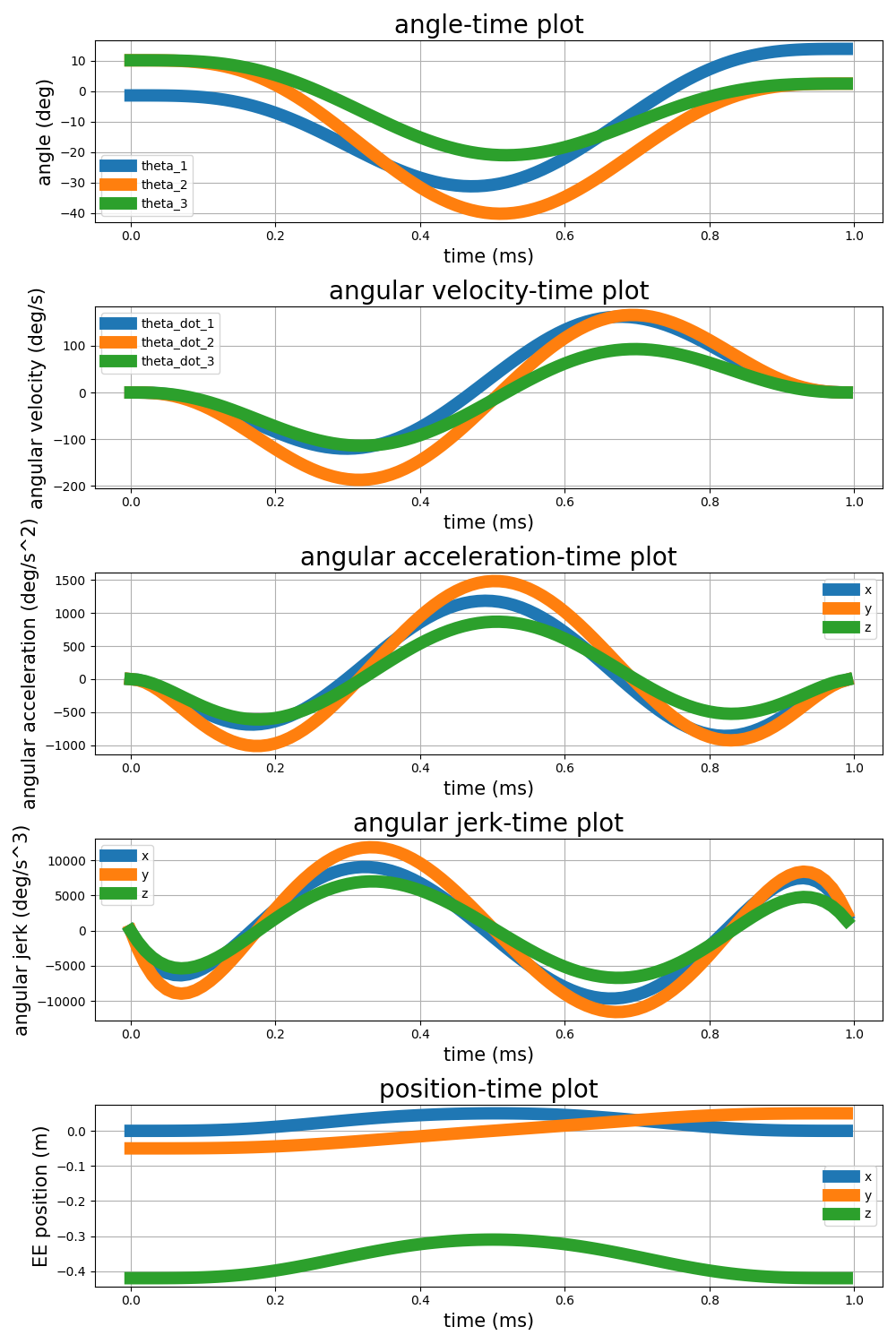
The result of this method is shown in the figure below. As explained, the advantage of this method compared to 3-4-5 interpolating polynomial is that the jerk is bounded at the initial and final points.

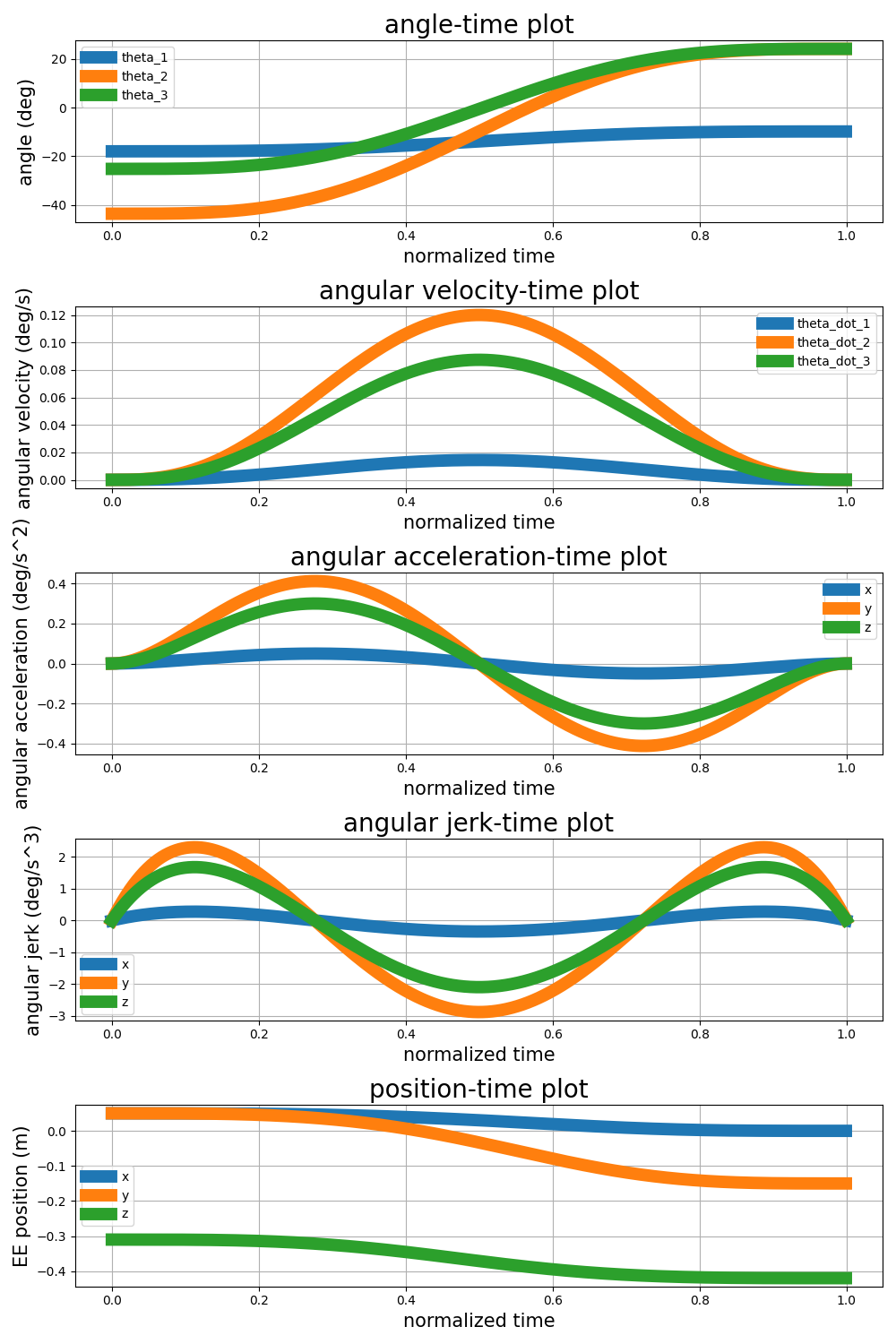
Discussion:

The 4-5-6-7 interpolating polynomial offers an improvement over the 3-4-5 interpolating polynomial by incorporating higher-order terms. The code can be found in the path planning file in the function point_to_point_4567

Trapezoidal method

---

Math::

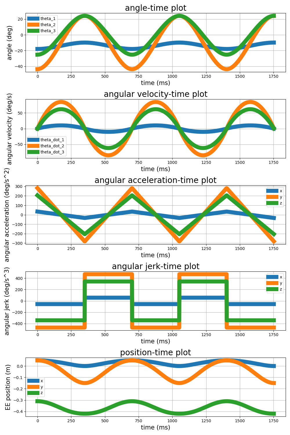
Like the previous methods, the goal here is to basically use a trapezoidal diagram as a way to interpolate the velocity profile between the values of $\theta^I$ and $\theta^F$. In this instance we call them $p$ and $p_0$. The trapezoidal diagram is defined as the following formula:

$$ \dot{p} = v = \begin{cases} at & t_0 \leq t < t_1 \\ V_{max} & t_1 \leq t < t_2 \\ -at & t_2 \leq t \leq t_3 \end{cases} $$

For the sake of simplicity we say that $t_0 = 0, t_1 = T/3, t_2 = 2T/3, t_3 = T$. Here's the result:

$$ \ddot{p} = a = \begin{cases} a & 0 \leq t < \frac{1}{3} T \\ 0 & \frac{2}{3} T \leq t < \frac{1}{3} T \\ -a & \frac{2}{3} T \leq t < T \\ \end{cases} \quad \quad \dot{p} = v = \begin{cases} at & 0 \leq t < \frac{1}{3} T \\ V_{max} & \frac{2}{3} T \leq t < \frac{1}{3} T \\ -at & \frac{2}{3} T \leq t < T \\ \end{cases} $$

Since $v_{max}$ is given to us as a limitation of our DPR, we use that value to calculate acceleration.

$$v_{max} = a.t_{t=\frac{1}{3} T} \rightarrow a = \frac{3v_{max}}{T}$$

Implementing this sequence with a Python script, we can get the results show as below [10]:

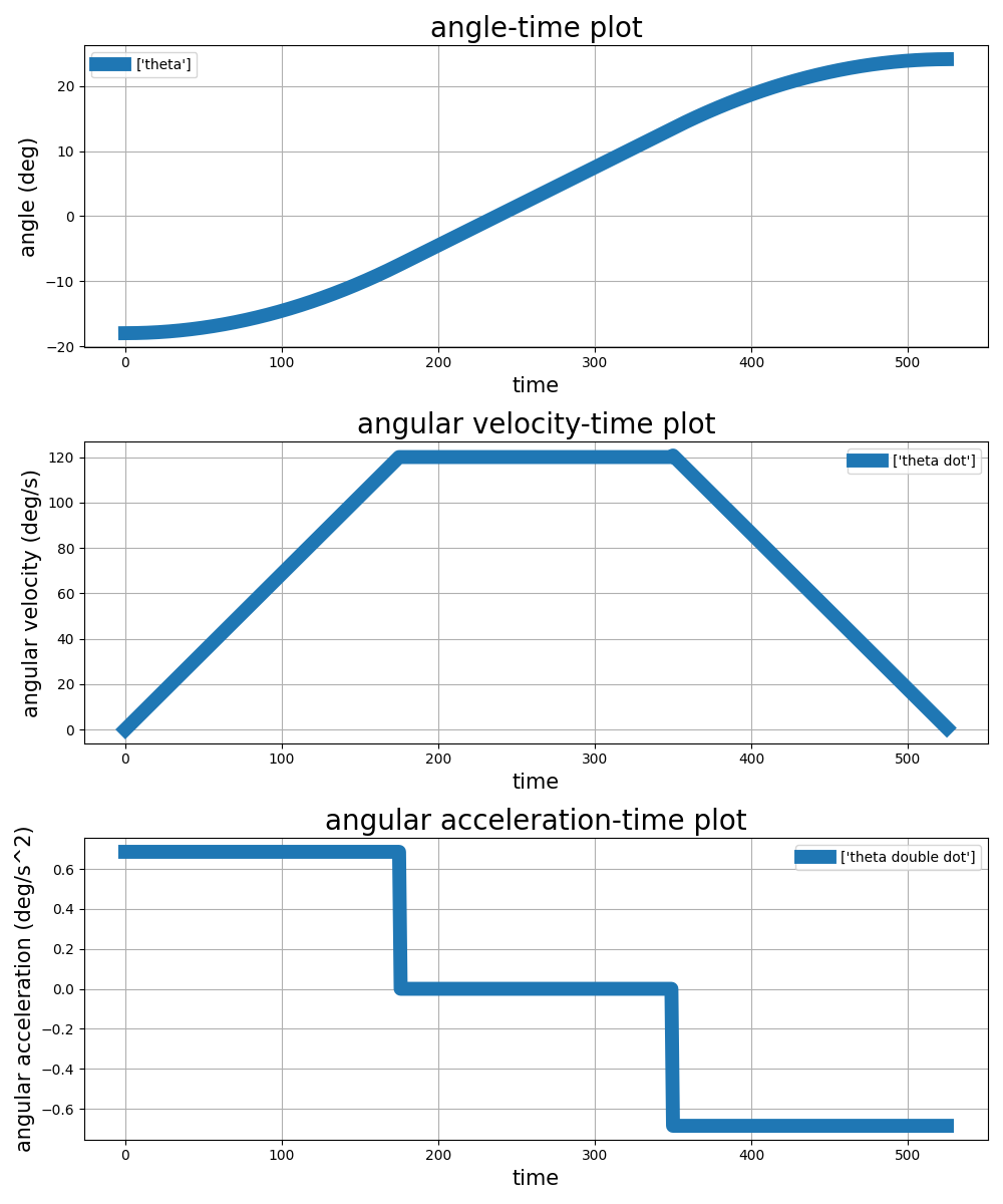
Discussion::

This method has the same problem of 3-4-5 method, but instead of start and finishing point, the problem is at $T/3$ and $2T/3$. The code can be found in the path planning file in the function trapezoidal_ptp

2.2 - Multi-Point Trajectory Planning

---

Multi-Point Trajectory Planning involves generating a path that include multiple target locations.

Higher Order Polynomials

---

Math

Remember how in the 4-5-6-7 interpolating polynomial we used a 7th order polynomial to constraint the jerk, acceleration, velocity and position of two points? In theory we can do that with any number of points. say we have $n+1$ points to interlpolate, and we also have the following constraints:

• initial and final velocity equals zero
• initial and final acceleration equals zero
• initial and final jerk equals zero

this means we'll be having $n+7$ overall conditions ($n+1$ points and 6 above conditions) that can be interpolated through a $n+6$th-order polynomial. Let's solve an example for a 3-point polynomial (which will have us solving an 8th-order polynomial to solve)

let's say we have the polynomial as:

$$ q(\tau) = a_8\tau^8 + \dots + a_1\tau + a_0 $$

and the conditions are for the polynomial $q$ to hit $q_0$, $q_1$ and $q_2$ and have initial and final velocity, acceleration and jerk equal to zero.

$$ \begin{cases} q(0) = q_0, \quad q(0.5) = q_1, \quad q(1) = q_2 \\ \dot{q}(0) = 0, \quad \dot{q}(1) = 0 \\ \ddot{q}(0) = 0, \quad \ddot{q}(1) = 0 \\ \dddot{q}(0) = 0 , \quad \dddot{q}(1) = 0 \end{cases} $$

These conditions will give us 9 equations as well as 9 coefficients to calculate which make up a system of linear equations. the equation solution is uploaded in this file and the final answers are:

$$ \begin{cases} a_0 = q_0 \\ a_1 = 0 \\ a_2 = 0 \\ a_3 = 0 \\ a_4 = 256q_1 - 163q_0 - 93q_2 \\ a_5 = 596q_0 - 1024q_1 + 428q_2 \\ a_6 = 1536q_1 - 838q_0 - 698q_2 \\ a_7 = 532q_0 - 1024q_1 + 492q_2 \\ a_8 = 256q_1 - 128q_0 - 128q_2 \end{cases} $$

Discussion

Using this method isn't all that appreciated anyways because for the larger numder of points we'll have some problems. Here are some of those problems listed:

• Less Sensitivity to Data Perturbations: High-degree polynomials are highly sensitive to changes in data points. Even small adjustments in the input data can significantly affect the resulting polynomial.
• Avoiding Overfitting: High-degree polynomials can lead to overfitting the data, capturing noise rather than the underlying trend.
• Numerical Efficiency: Solving systems of equations involving high-degree polynomials can be computationally expensive and may lead to numerical issues. In contrast, solving cubic splines is relatively efficient and numerically stable.
• Local Control: adding or removing a point in this method of high-order polynomial means recalculating the whole path instead of just one segment.

The method is implemented in this file in the function higher_order_poly_3pt

Cubic-Spline

---

When provided with $n+1$ points, it is feasible to construct a unique interpolating polynomial of degree $n$. However, as the number of points increases, the computational burden becomes heavier. To address this, an alternative approach is to utilize n polynomials of degree $p$ instead. The selection of $p$ is based on the desired level of continuity for the spline. For instance, if one aims to achieve continuity of velocities and accelerations at the time instances $t_k$, where the transition between two consecutive segments takes place, a cubic polynomial with degree $p=3$ can be assumed.

$$q(t) = a_0 + a_1t + a_2t^2 + a_3t^3$$

The overall function is given by

$$s(t) = \lbrace q_k(t), t\in [t_k, t_{k+1}], k=0, ..., n-1 \rbrace $$

$$ q_k(t) = a_{k0} + a_{k1}t + a_{k2}t^2 + a_{k3}t^3$$

By adopting this approach, it becomes essential to calculate four coefficients for each polynomial. Given that $n$ polynomials are required to define a trajectory using $n+1$ points, the total number of coefficients to be determined amounts to $4n$. To address this challenge, the following conditions need to be taken into account. Adding up the conditions that we have, $2n$ conditions for following the points, $n -1$ conditions for the continuity of velocities, and $n-1$ conditions for the continuity of accelerations, it can be seen that there are $4n-2$ conditions, in comparison to the $4n$ constants. The two degrees of freedom can be used for extra conditions such as:

• The initial and final velocities
• The initial and final accelerations
• The periodic conditions for velocity and acceleration
• The continuity of jerk

We assume assigned initial and final velocities

For given the points of $(t_k, q_k)$ for $k=0, ..., n$ we'll want to calculate: $$s(t) = \lbrace q_k(t), t\in[t_k, t_{k+1}], k=0, ..., n-1 \rbrace$$ $$q_k(t) = a_{k0} + a_{k1}(t-t_k) + a_{k2}(t-t_k)^2 + a_{k3}(t-t_k)^3$$

The conditions will be:

$$ \begin{cases} q_k(t_k) = q_k, \quad q_k(t_{k+1}) = q_{k+1}, & k=0, ..., n-1 \\ \dot{q_k} (t_{k+1}) = \dot{q_{k+1}}(t_{k+1})=v_{k+1}, & k=0, ..., n-2\\ \ddot{q_k} (t_{k+1}) = \ddot{q_{k+1}} (t_{k+1}), & k=0, ..., n-2\\ \dot{q_0} (t_0) = v_0, \quad \dot{q_{n-1}} (t_n) = v_n & \\ \end{cases} $$

solution

The coefficient $a_{k,i}$ can be computed with the following steps:

if we consider each velocity at time $t_k$ to be known:

$$ \begin{cases} q_k(t_k) = a_{k0}, & = q_k \\ \dot{q_k} (t_k) = a_{k1}, & = v_k \\ q_k(t_{k+1}) = a_{k0} + a_{k1} T_k + a_{k2} T^2_k + a_{k3}T^3_k, & = q_{k+1} \\ \dot{q_k} (t_{k+1}) = a_{k1} + 2a_{k2} T_k + 3 a_{k3} T^2_k, & = v_{k+1} \\ \end{cases} $$

Where $T_k = t_{k+1} - t_k$. Solving the above equations we have:

$$ \begin{cases} a_{k,0} = q_k\\ a_{k,1} = v_k\\ a_{k,2} = \frac{1}{T_k} [\frac{3(q_{k+1} - q_k)}{T_k} - 2v_k - v_{k+1}] \\ a_{k,3} = \frac{1}{T^2_k} [\frac{2(q_k - q_{k+1})}{T_k} + v_k + v_{k+1}] \\ \end{cases} $$

But this is for when the velocities of the points are known, which they are not (except the initial and final points). So the velocities have to be calculated, in this instance we use the continuity conditions of acceleration:

Velocities can be found with a matrix of $v = A^{-1}c$. Where:

$$ A = \begin{bmatrix} 2(T_0+T_1) & T_0 & 0 & ... & & 0 \\ T_2 & 2(T_1+T_2) & T_1 & 0 & & \vdots \\ 0 & & \ddots & & & 0 \\ \vdots & & & T_{n-2} & 2(T_{n-3}+T_{n-2}) & T_{n-3} \\ 0 & \dots & & 0 & T_{n-1} & 2(T_{n-2} + T_{n-1}) \\ \end{bmatrix} $$

$$ c = \begin{bmatrix} \frac{3}{T_0T_1} \left[ T^2_0(q_2 - q_1) + T^2_1(q_1 - q_0) \right] - T_1 v_0 \\ \frac{3}{T_1T_2} \left[ T^2_1(q_3 - q_2) + T^2_2(q_2 - q_1) \right] \\ \vdots \\ \frac{3}{T_{n-3}T_{n-2}} \left[ T^2_{n-3}(q_{n-1} - q_{n-2}) + T^2_{n-2}(q_{n-2} - q_{n-3}) \right] \\ \frac{3}{T_{n-2}T_{n-1}} \left[ T^2_{n-2}(q_n - q_{n-1}) + T^2_{n-1}(q_{n-1} - q_{n-2}) \right] - T_{n-2}v_n \\ \end{bmatrix} $$

$$ v = \begin{bmatrix} v_1 \\ v_2 \\ \vdots \\ v_{n-2} \\ v_{n-1} \\ \end{bmatrix} $$

Thus we have the velocities and the problem is solved. (for more details go to reference [10] Chapter 4.4). The implementation of this problem is coded in this python file and the results are:

Improved Cubic spline

---

RESEARCH

first method: intial and final zero acceleration

for more control over the start and finishing points we can use 4-th order polynomial for the start and finishing points. so instead of using n polynomials with an order of 3, we'll use n-2 polynomials with order of 3 and two polynmials with an order of 4. the first and final polynomials so to speak. This will give us two more constants hence, we can apply two more constraints.

second method: smooth acceleration curve

Another way of imporvemnt is to use p=4 altogether. this requires that the calculations be re-done in a similar manner to the previous section. of course one of the polynomials have to be p=5. either first or last polynomial so to speak. because the number of constrains we want for $n+1$ points are:

• $2n$ constraints for the positions
• $n-1$ constraints for the velocity continuity
• $n-1$ constraints for the acceleration continuity
• $n-1$ constraints for the jerk continuity
• $2$ constraints for initial and final velocity
• $2$ constraints for initial and final acceleration

that adds up to $5n+1$ constants. and since if we have n polynomials with the order of 4, we're going to get $5n$ constants. in order to add a constant, we can just put one of the polynomials a 5-th order.

First Method: Setting initial and final acceleration to zero Second Method: Continous Jerk Profile

Multi-Point Trapezoidal

---

We talked about the trapezoidal method in one of the point-to-point methods, but now we want to use it as a multi-point method. we already know about the 3 phases in trapezoidal. Assume that we want to use point-to-point interpolation on multiple points. What's the problem with that? it's the fact that the end effector will stop at all of the points that we want to hit. meaning if we define our points as $P_0, ..., P_n$, and we use point-to-point trajectory planning to go from $P_0$ to $P_1$ and from $P_1$ to $P_2$ and so on and so forth, the end effector will stop at each of the points (in some cases that might be what we want to do but in most cases that highly inefficient). but for now let's implement this for point-to-point trapezoidal. our first goal is to implement something like the figure (a) from the two diagrams about (Reference for picture is ref [10] - Part 3.2.4) - Hence the trapezoidal will reduce to a trianlge for us to hit the max velocity and then immediately enter the deceleration phase. the calculation will look like:

$$ \ddot{p} = a(t) = \begin{cases} a & 0 \leq t < T/2 \\ -a & T/2 \leq t \leq T \end{cases} $$

$$ \dot{p} = v(t) = \begin{cases} at & 0 \leq t < T/2 \\ -at & T/2 \leq t \leq T \end{cases} $$

$$ p(t) = \begin{cases} a\frac{t^2}{2} + p_0 & 0 \leq t < T/2 \\ \left[v_{max} \frac{t}{2} - 0.5v(t)(T-t)\right] + p_0 & T/2 \leq t \leq T \end{cases} $$

But since $v_{max} = \frac{T}{2}a$ and $p_{final} = v_{max}\times \frac{T}{2} + p_0$ and we're given the values for $a, p_{fina}, p_0$ with these two equations values for $T$ and $v_{max}$ can be found

$$ \begin{cases} T = \sqrt{(p_{final} - p_0)\frac{4}{a}} \\ v_{max} = a \frac{T}{2} \end{cases} $$

I wish it was as easy as this though. since we have three motors we have to synchronize them first and then we can generate the velocity profile.

2.3 - Visualizing The Theoretical Results

---

3D Animation for results of the sampled data of generated trajectories.

4-5-6-7 interpolating polynomial

4-5-6-7.trajectory.mp4

cubic spline results

cubic.spline.mp4

3 - Experimental Implementation

---

In this section I'll be implementing the theories studied in the previous section on the Delta Parallel Robot developed at the Human and Robot Interaction Laboratory - University of Tehran. The code of controlling the Delta Parallel Robot can be found in This Link

References

---

[1] doi: /10.1007/978-3-030-03538-9 23
[2] doi: 10.32629/jai.v5i1.505
[3] doi: 10.1109/CRC.2017.38
[4] doi: 10.3390/app9214491
[5] doi: 10.1007/s00170-019-04421-7
[6] doi: 10.3390/app12168145
[7] Research of Trajectory Planning for Delta Parallel Robots, 2013 International Conference on Mechatronic Sciences, Electric Engineering and Computer (MEC)
[8] doi: 10.1007/s11786-012-0123-8
[9] Fundamentals of Robotic Mechanical Systems Theory, Methods, and Algorithms, Fourth Edition by Jorge Angeles
[10] Trajectory Planning for Automatic Machines and Robots by Luigi Biagiotti, Claudio Melchiorri