OSPRay

This is release v3.1.0 of Intel® OSPRay. For changes and new features see the changelog. Visit http://www.ospray.org for more information.

OSPRay Overview

Intel® OSPRay is an open source, scalable, and portable ray tracing engine for high-performance, high-fidelity visualization on Intel Architecture CPUs, Intel Xe GPUs, and ARM64 CPUs. OSPRay is part of the Intel oneAPI Rendering Toolkit and is released under the permissive Apache 2.0 license.

The purpose of OSPRay is to provide an open, powerful, and easy-to-use rendering library that allows one to easily build applications that use ray tracing based rendering for interactive applications (including both surface- and volume-based visualizations). OSPRay runs on anything from laptops, to workstations, to compute nodes in HPC systems.

OSPRay internally builds on top of Intel Embree, Intel Open VKL, and Intel Open Image Denoise. The CPU implementation is based on Intel ISPC (Implicit SPMD Program Compiler) and fully exploits modern instruction sets like Intel SSE4, AVX, AVX2, AVX-512 and NEON to achieve high rendering performance. Hence, a CPU with support for at least SSE4.1 is required to run OSPRay on x86_64 architectures, or a CPU with support for NEON is required to run OSPRay on ARM64 architectures.

OSPRay’s GPU implementation (beta status) is based on the SYCL cross-platform programming language implemented by Intel oneAPI Data Parallel C++ (DPC++) and currently supports Intel Arc™ GPUs on Linux and Windows, and Intel Data Center GPU Flex and Max Series on Linux, exploiting ray tracing hardware support.

OSPRay Support and Contact

OSPRay is under active development, and though we do our best to guarantee stable release versions a certain number of bugs, as-yet-missing features, inconsistencies, or any other issues are still possible. For any such requests or findings please use OSPRay’s GitHub Issue Tracker (or, if you should happen to have a fix for it, you can also send us a pull request).

To receive release announcements simply “Watch” the OSPRay repository on GitHub.

Building and Finding OSPRay

The latest OSPRay sources are always available at the OSPRay GitHub repository. The default master branch should always point to the latest bugfix release.

Prerequisites

OSPRay currently supports Linux, Mac OS X, and Windows. In addition, before you can build OSPRay you need the following prerequisites:

• You can clone the latest OSPRay sources via:

  git clone https://github.com/ospray/ospray.git

• To build OSPRay you need CMake, any form of C++11 compiler (we recommend using GCC, but also support Clang, MSVC, and Intel® C++ Compiler (icc)), and standard Linux development tools.

• Additionally you require a copy of the Intel® Implicit SPMD Program Compiler (ISPC), version 1.23.0 or later. Please obtain a release of ISPC from the ISPC downloads page. If ISPC is not found by CMake its location can be hinted with the variable ispcrt_DIR.

• OSPRay builds on top of the Intel oneAPI Rendering Toolkit common library (rkcommon). The library provides abstractions for tasking, aligned memory allocation, vector math types, among others. For users who also need to build rkcommon, we recommend the default the Intel Threading Building Blocks (TBB) as tasking system for performance and flexibility reasons. TBB must be built from source when targeting ARM CPUs, or can be built from source as part of the superbuild. Alternatively you can set CMake variable RKCOMMON_TASKING_SYSTEM to OpenMP or Internal.

• OSPRay also heavily uses Intel Embree, installing version 4.3.1 or newer is required. If Embree is not found by CMake its location can be hinted with the variable embree_DIR.

• OSPRay supports volume rendering (enabled by default via OSPRAY_ENABLE_VOLUMES), which heavily uses Intel Open VKL, version 2.0.1 or newer is required. If Open VKL is not found by CMake its location can be hinted with the variable openvkl_DIR, or disable OSPRAY_ENABLE_VOLUMES.

• OSPRay also provides an optional module implementing the denoiser image operation, which is enabled by OSPRAY_MODULE_DENOISER. This module requires Intel Open Image Denoise in version 2.2.0 or newer. You may need to hint the location of the library with the CMake variable OpenImageDenoise_DIR.

• For the optional MPI modules (enabled by OSPRAY_MODULE_MPI), which provide the mpiOffload and mpiDistributed devices, you need an MPI library and Google Snappy.

• The optional example application, the test suit and benchmarks need some version of OpenGL and GLFW as well as GoogleTest and Google Benchmark

Depending on your Linux distribution you can install these dependencies using yum or apt-get. Some of these packages might already be installed or might have slightly different names.

Type the following to install the dependencies using yum:

sudo yum install cmake.x86_64
sudo yum install tbb.x86_64 tbb-devel.x86_64

Type the following to install the dependencies using apt-get:

sudo apt-get install cmake-curses-gui
sudo apt-get install libtbb-dev

Under Mac OS X these dependencies can be installed using MacPorts:

sudo port install cmake tbb

Under Windows please directly use the appropriate installers for CMake, TBB, ISPC (for your Visual Studio version) and Embree.

Additional Prerequisites for GPU Build

To build OSPRay’s GPU module you need

• a SYCL compiler, either the open source oneAPI DPC++ Compiler 2023-10-26 or the latest Intel oneAPI DPC++/C++ Compiler
• a recent CMake, version 3.25.3 or higher
• the oneAPI Level Zero Loader v1.12.0 development packages
  • On Linux Ubuntu 22.04 there are prebuilt packages available for this: level-zero-devel and level-zero
  • Other Linux distributions require building these packages from source
  • On Windows, you can use the single package level-zero_<version>_win-sdk; note you will need to set the environment variable LEVEL_ZERO_ROOT to the location of the SDK

CMake Superbuild

For convenience, OSPRay provides a CMake Superbuild script which will pull down OSPRay’s dependencies and build OSPRay itself. By default, the result is an install directory, with each dependency in its own directory.

Run with:

mkdir build
cd build
cmake [<OSPRAY_SOURCE_DIR>/scripts/superbuild]
cmake --build .

On Windows make sure to select a 64bit generator, e.g.

cmake -G "Visual Studio 17 2022" [<OSPRAY_SOURCE_DIR>/scripts/superbuild]

The resulting install directory (or the one set with CMAKE_INSTALL_PREFIX) will have everything in it, with one subdirectory per dependency.

CMake options to note (all have sensible defaults):

CMAKE_INSTALL_PREFIX
will be the root directory where everything gets installed.

BUILD_JOBS
sets the number given to make -j for parallel builds.

INSTALL_IN_SEPARATE_DIRECTORIES
toggles installation of all libraries in separate or the same directory.

BUILD_OPENVKL
whether to enable volume rendering via Open VKL

BUILD_EMBREE_FROM_SOURCE
set to OFF will download a pre-built version of Embree.

BUILD_OIDN_FROM_SOURCE
set to OFF will download a pre-built version of Open Image Denoise.

OIDN_VERSION
determines which version of Open Image Denoise to pull down.

BUILD_OSPRAY_MODULE_MPI
set to ON to build OSPRay’s MPI module for data-replicated and distributed parallel rendering on multiple nodes.

BUILD_GPU_SUPPORT
enables beta GPU support, fetching the SYCL variants of the dependencies and builds OSPRAY_MODULE_GPU

BUILD_TBB_FROM_SOURCE
set to ON to build TBB from source (required for ARM support). The default setting is OFF.

For the full set of options, run:

ccmake [<OSPRAY_SOURCE_DIR>/scripts/superbuild]

or

cmake-gui [<OSPRAY_SOURCE_DIR>/scripts/superbuild]

Cross-Compilation with the Superbuild

The superbuild can be passed a CMake Toolchain file to configure for cross-compilation. This is done by passing the toolchain file when running cmake. When cross compiling it is also likely that you’ll want to build TBB and Embree from source to ensure they’re built for the correct target, rather than the target the Github binaries are built for. It may also be necessary to disable specific ISAs for the target by passing BUILD_ISA_<ISA_NAME>=OFF as well.

mkdir build
cd build
cmake --toolchain [toolchain_file.cmake] [path/to/this/directory]
    -DBUILD_TBB_FROM_SOURCE=ON \
    -DBUILD_EMBREE_FROM_SOURCE=ON \
    <other arguments>

While OSPRay supports ARM natively, it may be desirable to cross-compile it for x86_64 to run in Rosetta depending on the application integrating OSPRay. This can be done using the toolchain file toolchains/macos-rosetta.cmake, and by disabling all non-SSE ISAs when building. This can also be done by launching an x86_64 bash shell and then compiling as usual in this environment, which will cause the compilation chain to target x86_64. The BUILD_ISA_<ISA NAME>=OFF flags should be passed to disable all ISAs besides SSE4 for Rosetta:

arch -x86_64 bash
mkdir build
cd build
cmake [path/to/this/directory]
    -DBUILD_TBB_FROM_SOURCE=ON \
    -DBUILD_EMBREE_FROM_SOURCE=ON \
    -DBUILD_ISA_AVX=OFF \
    -DBUILD_ISA_AVX2=OFF \
    -DBUILD_ISA_AVX512=OFF \
    <other arguments>

Standard CMake Build

Compiling OSPRay on Linux and Mac OS X

Assuming the above requisites are all fulfilled, building OSPRay through CMake is easy:

• Create a build directory, and go into it

  mkdir ospray/build
  cd ospray/build

  (We do recommend having separate build directories for different configurations such as release, debug, etc.).

• The compiler CMake will use will default to whatever the CC and CXX environment variables point to. Should you want to specify a different compiler, run cmake manually while specifying the desired compiler. The default compiler on most linux machines is gcc, but it can be pointed to clang instead by executing the following:

  cmake -DCMAKE_CXX_COMPILER=clang++ -DCMAKE_C_COMPILER=clang ..

  CMake will now use Clang instead of GCC. If you are OK with using the default compiler on your system, then simply skip this step. Note that the compiler variables cannot be changed after the first cmake or ccmake run.

• Open the CMake configuration dialog

  ccmake ..

• Make sure to properly set build mode and enable the components you need, etc.; then type ’c’onfigure and ’g’enerate. When back on the command prompt, build it using

  make

• You should now have libospray.[so,dylib] as well as a set of example applications.

Compiling OSPRay on Windows

On Windows using the CMake GUI (cmake-gui.exe) is the most convenient way to configure OSPRay and to create the Visual Studio solution files:

• Browse to the OSPRay sources and specify a build directory (if it does not exist yet CMake will create it).

• Click “Configure” and select as generator the Visual Studio version you have; OSPRay needs “Visual Studio 15 2017 Win64” or newer, 32
  bit builds are not supported, e.g., “Visual Studio 17 2022”.

• If the configuration fails because some dependencies could not be found then follow the instructions given in the error message, e.g., set the variable embree_DIR to the folder where Embree was installed and openvkl_DIR to where Open VKL was installed.

• Optionally change the default build options, and then click “Generate” to create the solution and project files in the build directory.

• Open the generated OSPRay.sln in Visual Studio, select the build configuration and compile the project.

Alternatively, OSPRay can also be built without any GUI, entirely on the console. In the Visual Studio command prompt type:

cd path\to\ospray
mkdir build
cd build
cmake -G "Visual Studio 17 2022" [-D VARIABLE=value] ..
cmake --build . --config Release

Use -D to set variables for CMake, e.g., the path to Embree with “-D embree_DIR=\path\to\embree”.

You can also build only some projects with the --target switch. Additional parameters after “--” will be passed to msbuild. For example, to build in parallel only the OSPRay library without the example applications use

cmake --build . --config Release --target ospray -- /m

Finding an OSPRay Install with CMake

Client applications using OSPRay can find it with CMake’s find_package() command. For example,

find_package(ospray 3.0.0 REQUIRED)

finds OSPRay via OSPRay’s configuration file osprayConfig.cmake¹. Once found, the following is all that is required to use OSPRay:

target_link_libraries(${client_target} ospray::ospray)

This will automatically propagate all required include paths, linked libraries, and compiler definitions to the client CMake target (either an executable or library).

Advanced users may want to link to additional targets which are exported in OSPRay’s CMake config, which includes all installed modules. All targets built with OSPRay are exported in the ospray:: namespace, therefore all targets locally used in the OSPRay source tree can be accessed from an install. For example, ospray_module_cpu can be consumed directly via the ospray::ospray_module_cpu target. All targets have their libraries, includes, and definitions attached to them for public consumption (please report bugs if this is broken!).

Documentation

The following API documentation of OSPRay can also be found as a pdf document.

For a deeper explanation of the concepts, design, features and performance of OSPRay also have a look at the IEEE Vis 2016 paper “OSPRay – A CPU Ray Tracing Framework for Scientific Visualization” (49MB, or get the smaller version 1.8MB). The slides of the talk (5.2MB) are also available.

OSPRay API

To access the OSPRay API you first need to include the OSPRay header

#include "ospray/ospray.h"

where the API is compatible with C99 and C++.

Initialization and Shutdown

To use the API, OSPRay must be initialized with a “device”. A device is the object which implements the API. Creating and initializing a device can be done in either of two ways: command line arguments using ospInit or manually instantiating a device and setting parameters on it.

Command Line Arguments

The first is to do so by giving OSPRay the command line from main() by calling

OSPError ospInit(int *argc, const char **argv);

OSPRay parses (and removes) its known command line parameters from your application’s main function. For an example see the tutorial. For possible error codes see section Error Handling and Status Messages. It is important to note that the arguments passed to ospInit are processed in order they are listed. The following parameters (which are prefixed by convention with “--osp:”) are understood:

Parameter	Description
--osp:debug	enables various extra checks and debug output, and disables multi-threading
--osp:num-threads=<n>	use n threads instead of per default using all detected hardware threads
--osp:log-level=<str>	set logging level; valid values (in order of severity) are none, error, warning, info, and debug
--osp:warn-as-error	send warning and error messages through the error callback, otherwise send warning messages through the message callback; must have sufficient logLevel to enable warnings
--osp:verbose	shortcut for --osp:log-level=info and enable debug output on cout, error output on cerr
--osp:vv	shortcut for --osp:log-level=debug and enable debug output on cout, error output on cerr
--osp:load-modules=<name>[,...]	load one or more modules during initialization; equivalent to calling ospLoadModule(name)
--osp:log-output=<dst>	convenience for setting where status messages go; valid values for dst are cerr and cout
--osp:error-output=<dst>	convenience for setting where error messages go; valid values for dst are cerr and cout
--osp:device=<name>	use name as the type of device for OSPRay to create; e.g., --osp:device=cpu gives you the default cpu device; Note if the device to be used is defined in a module, remember to pass --osp:load-modules=<name> first
--osp:set-affinity=<n>	if 1, bind software threads to hardware threads; 0 disables binding; default is 0
--osp:device-params=<param>:<value>[,...]	set one or more other device parameters; equivalent to calling ospDeviceSet*(param, value)

Command line parameters accepted by OSPRay’s ospInit.

Manual Device Instantiation

The second method of initialization is to explicitly create the device and possibly set parameters. This method looks almost identical to how other objects are created and used by OSPRay (described in later sections). The first step is to create the device with

OSPDevice ospNewDevice(const char *type);

where the type string maps to a specific device implementation. OSPRay always provides the “cpu” device, which maps to a fast, local CPU implementation. Other devices can also be added through additional modules, such as distributed MPI device implementations. See next Chapter for details.

Once a device is created, you can call

void ospDeviceSetParam(OSPObject, const char *id, OSPDataType type, const void *mem);

to set parameters on the device. The semantics of setting parameters is exactly the same as ospSetParam, which is documented below in the parameters section. The following parameters can be set on all devices:

Type	Name	Description
int	numThreads	number of threads which OSPRay should use
uint	logLevel	logging level; valid values (in order of severity) are OSP_LOG_NONE, OSP_LOG_ERROR, OSP_LOG_WARNING, OSP_LOG_INFO, and OSP_LOG_DEBUG
string	logOutput	convenience for setting where status messages go; valid values are cerr and cout
string	errorOutput	convenience for setting where error messages go; valid values are cerr and cout
bool	debug	set debug mode; equivalent to logLevel=debug and numThreads=1
bool	warnAsError	send warning and error messages through the error callback, otherwise send warning messages through the message callback; must have sufficient logLevel to enable warnings
bool	setAffinity	bind software threads to hardware threads if set to 1; 0 disables binding omitting the parameter will let OSPRay choose

Parameters shared by all devices.

Once parameters are set on the created device, the device must be committed with

void ospDeviceCommit(OSPDevice);

To use the newly committed device, you must call

void ospSetCurrentDevice(OSPDevice);

This then sets the given device as the object which will respond to all other OSPRay API calls.

Device handle lifetimes are managed with two calls, the first which increments the internal reference count to the given OSPDevice

void ospDeviceRetain(OSPDevice)

and the second which decrements the reference count

void ospDeviceRelease(OSPDevice)

Users can change parameters on the device after initialization (from either method above), by calling

OSPDevice ospGetCurrentDevice();

This function returns the handle to the device currently used to respond to OSPRay API calls, where users can set/change parameters and recommit the device. If changes are made to the device that is already set as the current device, it does not need to be set as current again. Note this API call will increment the ref count of the returned device handle, so applications must use ospDeviceRelease when finished using the handle to avoid leaking the underlying device object. If there is no current device set, this will return an invalid NULL handle.

When a device is created, its reference count is initially 1. When a device is set as the current device, it internally has its reference count incremented. Note that ospDeviceRetain and ospDeviceRelease should only be used with reference counts that the application tracks: removing reference held by the current set device should be handled by ospShutdown. Thus, ospDeviceRelease should only decrement the reference counts that come from ospNewDevice, ospGetCurrentDevice, and the number of explicit calls to ospDeviceRetain.

OSPRay allows applications to query runtime properties of a device in order to do enhanced validation of what device was loaded at runtime. The following function can be used to get these device-specific properties (attributes about the device, not parameter values)

int64_t ospDeviceGetProperty(OSPDevice, OSPDeviceProperty);

It returns an integer value of the queried property and the following properties can be provided as parameter:

OSP_DEVICE_VERSION
OSP_DEVICE_VERSION_MAJOR
OSP_DEVICE_VERSION_MINOR
OSP_DEVICE_VERSION_PATCH
OSP_DEVICE_SO_VERSION

Environment Variables

OSPRay’s generic device parameters can be overridden via environment variables for easy changes to OSPRay’s behavior without needing to change the application (variables are prefixed by convention with “OSPRAY_”):

Variable	Description
OSPRAY_NUM_THREADS	equivalent to --osp:num-threads
OSPRAY_LOG_LEVEL	equivalent to --osp:log-level
OSPRAY_LOG_OUTPUT	equivalent to --osp:log-output
OSPRAY_ERROR_OUTPUT	equivalent to --osp:error-output
OSPRAY_DEBUG	equivalent to --osp:debug
OSPRAY_WARN_AS_ERROR	equivalent to --osp:warn-as-error
OSPRAY_SET_AFFINITY	equivalent to --osp:set-affinity
OSPRAY_LOAD_MODULES	equivalent to --osp:load-modules, can be a comma separated list of modules which will be loaded in order
OSPRAY_DEVICE	equivalent to --osp:device:

Environment variables interpreted by OSPRay.

Note that these environment variables take precedence over values specified through ospInit or manually set device parameters.

Error Handling and Status Messages

The following errors are currently used by OSPRay:

Name	Description
OSP_NO_ERROR	no error occurred
OSP_UNKNOWN_ERROR	an unknown error occurred
OSP_INVALID_ARGUMENT	an invalid argument was specified
OSP_INVALID_OPERATION	the operation is not allowed for the specified object
OSP_OUT_OF_MEMORY	there is not enough memory to execute the command
OSP_UNSUPPORTED_CPU	the CPU is not supported (minimum ISA is SSE4.1 on x86_64 and NEON on ARM64)
OSP_VERSION_MISMATCH	a module could not be loaded due to mismatching version

Possible error codes, i.e., valid named constants of type OSPError.

These error codes are either directly return by some API functions, or are recorded to be later queried by the application via

OSPError ospDeviceGetLastErrorCode(OSPDevice);

A more descriptive error message can be queried by calling

const char* ospDeviceGetLastErrorMsg(OSPDevice);

Alternatively, the application can also register a callback function of type

typedef void (*OSPErrorCallback)(void *userData, OSPError, const char* errorDetails);

via

void ospDeviceSetErrorCallback(OSPDevice, OSPErrorCallback, void *userData);

to get notified when errors occur.

Applications may be interested in messages which OSPRay emits, whether for debugging or logging events. Applications can call

void ospDeviceSetStatusCallback(OSPDevice, OSPStatusCallback, void *userData);

in order to register a callback function of type

typedef void (*OSPStatusCallback)(void *userData, const char* messageText);

which OSPRay will use to emit status messages. By default, OSPRay uses a callback which does nothing, so any output desired by an application will require that a callback is provided. Note that callbacks for C++ std::cout and std::cerr can be alternatively set through ospInit or the OSPRAY_LOG_OUTPUT environment variable.

Applications can clear either callback by passing NULL instead of an actual function pointer.

Loading OSPRay Extensions at Runtime

OSPRay’s functionality can be extended via plugins (which we call “modules”), which are implemented in shared libraries. To load module name from libospray_module_<name>.so (on Linux and Mac OS X) or ospray_module_<name>.dll (on Windows) use

OSPError ospLoadModule(const char *name);

Modules are searched in OS-dependent paths. ospLoadModule returns OSP_NO_ERROR if the plugin could be successfully loaded.

Shutting Down OSPRay

When the application is finished using OSPRay (typically on application exit), the OSPRay API should be finalized with

void ospShutdown();

This API call ensures that the current device is cleaned up appropriately. Due to static object allocation having non-deterministic ordering, it is recommended that applications call ospShutdown before the calling application process terminates.

Objects

All entities of OSPRay (the renderer, volumes, geometries, lights, cameras, …) are a logical specialization of OSPObject and share common mechanism to deal with parameters and lifetime.

An important aspect of object parameters is that parameters do not get passed to objects immediately. Instead, parameters are not visible at all to objects until they get explicitly committed to a given object via a call to

void ospCommit(OSPObject);

at which time all previously additions or changes to parameters are visible at the same time. If a user wants to change the state of an existing object (e.g., to change the origin of an already existing camera) it is perfectly valid to do so, as long as the changed parameters are recommitted.

The commit semantic allow for batching up multiple small changes, and specifies exactly when changes to objects will occur. This can impact performance and consistency for devices crossing a PCI bus or across a network.

Note that OSPRay uses reference counting to manage the lifetime of all objects, so one cannot explicitly “delete” any object. Instead, to indicate that the application does not need and does not access the given object anymore, call

void ospRelease(OSPObject);

This decreases its reference count and if the count reaches 0 the object will automatically get deleted. Passing NULL is not an error. Note that every handle returned via the API needs to be released when the object is no longer needed, to avoid memory leaks.

Sometimes applications may want to have more than one reference to an object, where it is desirable for the application to increment the reference count of an object. This is done with

void ospRetain(OSPObject);

It is important to note that this is only necessary if the application wants to call ospRelease on an object more than once: objects which contain other objects as parameters internally increment/decrement ref counts and should not be explicitly done by the application.

Parameters

Parameters allow to configure the behavior of and to pass data to objects. However, objects do not have an explicit interface for reasons of high flexibility and a more stable compile-time API. Instead, parameters are passed separately to objects in an arbitrary order, and unknown parameters will simply be ignored (though a warning message will be posted). The following function allows adding various types of parameters with name id to a given object:

void ospSetParam(OSPObject, const char *id, OSPDataType type, const void *mem);

The valid parameter names for all OSPObjects and what types are valid are discussed in future sections.

Note that mem must always be a pointer to the object, otherwise accidental type casting can occur. This is especially true for pointer types (OSP_VOID_PTR and OSPObject handles), as they will implicitly cast to void *, but be incorrectly interpreted. To help with some of these issues, there also exist variants of ospSetParam for specific types, such as ospSetInt and ospSetVec3f in the OSPRay utility library (found in ospray_util.h). Note that half precision float parameters OSP_HALF, OSP_VEC[234]H are not supported.

Users can also remove parameters that have been explicitly set from ospSetParam. Any parameters which have been removed will go back to their default value during the next commit unless a new parameter was set after the parameter was removed. To remove a parameter, use

void ospRemoveParam(OSPObject, const char *id);

Data

OSPRay consumes data arrays from the application using a specific object type, OSPData. There are several components to describing a data array: element type, 1/2/3 dimensional striding, and whether the array is shared with the application or copied into opaque, OSPRay-owned memory.

Shared data arrays require that the application’s array memory outlives the lifetime of the created OSPData, as OSPRay is referring to application memory. Where this is not preferable, applications use opaque arrays to allow the OSPData to own the lifetime of the array memory. However, opaque arrays dictate the cost of copying data into it, which should be kept in mind.

Thus, the most efficient way to specify a data array from the application is to created a shared data array, which is done with

OSPData ospNewSharedData(const void *sharedData,
    OSPDataType,
    uint64_t numItems1,
    int64_t byteStride1 = 0,
    uint64_t numItems2 = 1,
    int64_t byteStride2 = 0,
    uint64_t numItems3 = 1,
    int64_t byteStride3 = 0,
    OSPDeleterCallback = NULL,
    void *userData = NULL);

The call returns an OSPData handle to the created array. The calling program guarantees that the sharedData pointer will remain valid for the duration that this data array is being used. The number of elements numItems must be positive (there cannot be an empty data object). The data is arranged in three dimensions, with specializations to two or one dimension (if some numItems are 1). The distance between consecutive elements (per dimension) is given in bytes with byteStride and can also be negative. If byteStride is zero it will be determined automatically (e.g., as sizeof(type)). Strides do not need to be ordered, i.e., byteStride2 can be smaller than byteStride1, which is equivalent to a transpose. However, if the stride should be calculated, then an ordering in dimensions is assumed to disambiguate, i.e., byteStride1 < byteStride2 < byteStride3.

An application can pass ownership of shared data to OSPRay (for example, when it temporarily created a modified version of its data only to make it compatible with OSPRay) by providing a deleter function that OSPRay will call whenever the time comes to deallocate the shared buffer. The deleter function has the following signature:

typedef void (*OSPDeleterCallback)(const void *userData, const void *sharedData);

where sharedData will receive the address of the buffer and userData will receive whatever additional state the function needs to perform the deletion (both provided to ospNewSharedData when sharing the data with OSPRay).

The enum type OSPDataType describes the different element types that can be represented in OSPRay; valid constants are listed in the table below.

Type / Name	Description
OSP_DEVICE	API device object reference
OSP_DATA	data reference
OSP_OBJECT	generic object reference
OSP_CAMERA	camera object reference
OSP_FRAMEBUFFER	framebuffer object reference
OSP_LIGHT	light object reference
OSP_MATERIAL	material object reference
OSP_TEXTURE	texture object reference
OSP_RENDERER	renderer object reference
OSP_WORLD	world object reference
OSP_GEOMETRY	geometry object reference
OSP_VOLUME	volume object reference
OSP_TRANSFER_FUNCTION	transfer function object reference
OSP_IMAGE_OPERATION	image operation object reference
OSP_STRING	C-style zero-terminated character string
OSP_CHAR, OSP_VEC[234]C	8 bit signed character scalar and [234]-element vector
OSP_UCHAR, OSP_VEC[234]UC	8 bit unsigned character scalar and [234]-element vector
OSP_SHORT, OSP_VEC[234]S	16 bit unsigned integer scalar and [234]-element vector
OSP_USHORT, OSP_VEC[234]US	16 bit unsigned integer scalar and [234]-element vector
OSP_INT, OSP_VEC[234]I	32 bit signed integer scalar and [234]-element vector
OSP_UINT, OSP_VEC[234]UI	32 bit unsigned integer scalar and [234]-element vector
OSP_LONG, OSP_VEC[234]L	64 bit signed integer scalar and [234]-element vector
OSP_ULONG, OSP_VEC[234]UL	64 bit unsigned integer scalar and [234]-element vector
OSP_HALF, OSP_VEC[234]H	16 bit half precision floating-point scalar and [234]-element vector (IEEE 754 binary16)
OSP_FLOAT, OSP_VEC[234]F	32 bit single precision floating-point scalar and [234]-element vector
OSP_DOUBLE, OSP_VEC[234]D	64 bit double precision floating-point scalar and [234]-element vector
OSP_BOX[1234]I	32 bit integer box (lower + upper bounds)
OSP_BOX[1234]F	32 bit single precision floating-point box (lower + upper bounds)
OSP_LINEAR[23]F	32 bit single precision floating-point linear transform ([23] vectors)
OSP_AFFINE[23]F	32 bit single precision floating-point affine transform (linear transform plus translation)
OSP_QUATF	32 bit single precision floating-point quaternion, in $(i, j, k, w)$ layout
OSP_VOID_PTR	raw memory address (only found in module extensions)

Valid named constants for OSPDataType.

If the elements of the array are handles to objects, then their reference counter is incremented.

An opaque OSPData with memory allocated by OSPRay is created with

OSPData ospNewData(OSPDataType,
    uint64_t numItems1,
    uint64_t numItems2 = 1,
    uint64_t numItems3 = 1);

To allow for (partial) copies or updates of data arrays use

void ospCopyData(const OSPData source,
    OSPData destination,
    uint64_t destinationIndex1 = 0,
    uint64_t destinationIndex2 = 0,
    uint64_t destinationIndex3 = 0);

which will copy the whole² content of the source array into destination at the given location destinationIndex. The OSPDataTypes of the data objects must match. The region to be copied must be valid inside the destination, i.e., in all dimensions, destinationIndex + sourceSize <= destinationSize. The affected region [destinationIndex, destinationIndex + sourceSize) is marked as dirty, which may be used by OSPRay to only process or update that sub-region (e.g., updating an acceleration structure). If the destination array is shared with OSPData by the application (created with ospNewSharedData), then

• the source array must be shared as well (thus ospCopyData cannot be used to read opaque data)
• if source and destination memory overlaps (aliasing), then behavior is undefined
• except if source and destination regions are identical (including matching strides), which can be used by application to mark that region as dirty (instead of the whole OSPData)

To add a data array as parameter named id to another object call also use

void ospSetObject(OSPObject, const char *id, OSPData);

Volumes

Volumes are volumetric data sets with discretely sampled values in 3D space, typically a 3D scalar field. To create a new volume object of given type type use

OSPVolume ospNewVolume(const char *type);

Note that OSPRay’s implementation forwards type directly to Open VKL, allowing new Open VKL volume types to be usable within OSPRay without the need to change (or even recompile) OSPRay.

Structured Regular Volume

Structured volumes only need to store the values of the samples, because their addresses in memory can be easily computed from a 3D position. A common type of structured volumes are regular grids.

Structured regular volumes are created by passing the type string “structuredRegular” to ospNewVolume. Structured volumes are represented through an OSPData 3D array data (which may or may not be shared with the application). The voxel data must be laid out in xyz-order³ and can be compact (best for performance) or can have a stride between voxels, specified through the byteStride1 parameter when creating the OSPData. Only 1D strides are supported, additional strides between scanlines (2D, byteStride2) and slices (3D, byteStride3) are not.

The parameters understood by structured volumes are summarized in the table below.

Type	Name	Default	Description
vec3f	gridOrigin	$(0, 0, 0)$	origin of the grid in object-space
vec3f	gridSpacing	$(1, 1, 1)$	size of the grid cells in object-space
OSPData	data		the actual voxel 3D data
bool	cellCentered	false	whether the data is provided per cell (as opposed to per vertex)
uint	filter	OSP_VOLUME_FILTER_LINEAR	filter used for reconstructing the field, also allowed is OSP_VOLUME_FILTER_NEAREST and OSP_VOLUME_FILTER_CUBIC
uint	gradientFilter	same as filter	filter used during gradient computations
float	background	NaN	value that is used when sampling an undefined region outside the volume domain

Configuration parameters for structured regular volumes.

The size of the volume is inferred from the size of the 3D array data, as is the type of the voxel values (currently supported are: OSP_UCHAR, OSP_SHORT, OSP_USHORT, OSP_HALF, OSP_FLOAT, and OSP_DOUBLE). Data can be provided either per cell or per vertex (the default), selectable via the cellCentered parameter (which will also affect the computed bounding box).

Structured Spherical Volume

Structured spherical volumes are also supported, which are created by passing a type string of “structuredSpherical” to ospNewVolume. The grid dimensions and parameters are defined in terms of radial distance $r$, inclination angle $\theta$, and azimuthal angle $\phi$, conforming with the ISO convention for spherical coordinate systems. The coordinate system and parameters understood by structured spherical volumes are summarized below.

Coordinate system of structured spherical volumes.

Type	Name	Default	Description
vec3f	gridOrigin	$(0, 0, 0)$	origin of the grid in units of $(r, \theta, \phi)$; angles in degrees
vec3f	gridSpacing	$(1, 180/dim.y, 360/dim.z)$	size of the grid cells in units of $(r, \theta, \phi)$, per default covering the full sphere; angles in degrees
OSPData	data		the actual voxel 3D data
uint	filter	OSP_VOLUME_FILTER_LINEAR	filter used for reconstructing the field, also allowed is OSP_VOLUME_FILTER_NEAREST
uint	gradientFilter	same as filter	filter used during gradient computations
float	background	NaN	value that is used when sampling an undefined region outside the volume domain

Configuration parameters for structured spherical volumes.

The dimensions $(r, \theta, \phi)$ of the volume are inferred from the size of the 3D array data, as is the type of the voxel values (currently supported are: OSP_UCHAR, OSP_SHORT, OSP_USHORT, OSP_HALF, OSP_FLOAT, and OSP_DOUBLE).

These grid parameters support flexible specification of spheres, hemispheres, spherical shells, spherical wedges, and so forth. The grid extents (computed as [gridOrigin, gridOrigin + (dimensions - 1) * gridSpacing]) however must be constrained such that:

• $r \geq 0$
• $0 \leq \theta \leq 180$
• $0 \leq \phi \leq 360$

Adaptive Mesh Refinement (AMR) Volume

OSPRay currently supports block-structured (Berger-Colella) AMR volumes. Volumes are specified as a list of blocks, which exist at levels of refinement in potentially overlapping regions. Blocks exist in a tree structure, with coarser refinement level blocks containing finer blocks. The cell width is equal for all blocks at the same refinement level, though blocks at a coarser level have a larger cell width than finer levels.

There can be any number of refinement levels and any number of blocks at any level of refinement. An AMR volume type is created by passing the type string “amr” to ospNewVolume.

Blocks are defined by three parameters: their bounds, the refinement level in which they reside, and the scalar data contained within each block.

Note that cell widths are defined per refinement level, not per block.

Type	Name	Default	Description
uint	method	OSP_AMR_CURRENT	OSPAMRMethod sampling method. Supported methods are:
			OSP_AMR_CURRENT
			OSP_AMR_FINEST
			OSP_AMR_OCTANT
float[]	cellWidth	NULL	array of each level’s cell width
box3i[]	block.bounds	NULL	data array of grid sizes (in voxels) for each AMR block
int[]	block.level	NULL	array of each block’s refinement level
OSPData[]	block.data	NULL	data array of OSPData containing the actual scalar voxel data, only OSP_FLOAT is supported as OSPDataType
vec3f	gridOrigin	$(0, 0, 0)$	origin of the grid
vec3f	gridSpacing	$(1, 1, 1)$	size of the grid cells
float	background	NaN	value that is used when sampling an undefined region outside the volume domain

Configuration parameters for AMR volumes.

Lastly, note that the gridOrigin and gridSpacing parameters act just like the structured volume equivalent, but they only modify the root (coarsest level) of refinement.

In particular, OSPRay’s / Open VKL’s AMR implementation was designed to cover Berger-Colella [1] and Chombo [2] AMR data. The method parameter above determines the interpolation method used when sampling the volume.

OSP_AMR_CURRENT
finds the finest refinement level at that cell and interpolates through this “current” level

OSP_AMR_FINEST
will interpolate at the closest existing cell in the volume-wide finest refinement level regardless of the sample cell’s level

OSP_AMR_OCTANT
interpolates through all available refinement levels at that cell. This method avoids discontinuities at refinement level boundaries at the cost of performance

Details and more information can be found in the publication for the implementation [3].

1. M.J. Berger and P. Colella, “Local adaptive mesh refinement for shock hydrodynamics.” Journal of Computational Physics 82.1 (1989): 64-84. DOI: 10.1016/0021-9991(89)90035-1
2. M. Adams, P. Colella, D.T. Graves, J.N. Johnson, N.D. Keen, T.J. Ligocki, D.F. Martin. P.W. McCorquodale, D. Modiano. P.O. Schwartz, T.D. Sternberg, and B. Van Straalen, “Chombo Software Package for AMR Applications – Design Document”, Lawrence Berkeley National Laboratory Technical Report LBNL-6616E.
3. I. Wald, C. Brownlee, W. Usher, and A. Knoll, “CPU volume rendering of adaptive mesh refinement data”. SIGGRAPH Asia 2017 Symposium on Visualization – SA ’17, 18(8), 1–8. DOI: 10.1145/3139295.3139305

Unstructured Volume

Unstructured volumes can have their topology and geometry freely defined. Geometry can be composed of tetrahedral, hexahedral, wedge or pyramid cell types. The data format used is compatible with VTK and consists of multiple arrays: vertex positions and values, vertex indices, cell start indices, cell types, and cell values. An unstructured volume type is created by passing the type string “unstructured” to ospNewVolume.

Sampled cell values can be specified either per-vertex (vertex.data) or per-cell (cell.data). If both arrays are set, cell.data takes precedence.

Similar to a mesh, each cell is formed by a group of indices into the vertices. For each vertex, the corresponding (by array index) data value will be used for sampling when rendering, if specified. The index order for a tetrahedron is the same as VTK_TETRA: bottom triangle counterclockwise, then the top vertex.

For hexahedral cells, each hexahedron is formed by a group of eight indices into the vertices and data values. Vertex ordering is the same as VTK_HEXAHEDRON: four bottom vertices counterclockwise, then top four counterclockwise.

For wedge cells, each wedge is formed by a group of six indices into the vertices and data values. Vertex ordering is the same as VTK_WEDGE: three bottom vertices counterclockwise, then top three counterclockwise.

For pyramid cells, each cell is formed by a group of five indices into the vertices and data values. Vertex ordering is the same as VTK_PYRAMID: four bottom vertices counterclockwise, then the top vertex.

To maintain VTK data compatibility, the index array may be specified with cell sizes interleaved with vertex indices in the following format: $n, id_1, ..., id_n, m, id_1, ..., id_m$. This alternative index array layout can be enabled through the indexPrefixed flag (in which case, the cell.type parameter must be omitted).

Type	Name	Default	Description
vec3f[]	vertex.position		data array of vertex positions
float[]	vertex.data		data array of vertex data values to be sampled
uint32[] / uint64[]	index		data array of indices (into the vertex array(s)) that form cells
bool	indexPrefixed	false	indicates that the index array is compatible to VTK, where the indices of each cell are prefixed with the number of vertices
uint32[] / uint64[]	cell.index		data array of locations (into the index array), specifying the first index of each cell
float[]	cell.data		data array of cell data values to be sampled
uint8[]	cell.type		data array of cell types (VTK compatible), only set if indexPrefixed = false false. Supported types are:
			OSP_TETRAHEDRON
			OSP_HEXAHEDRON
			OSP_WEDGE
			OSP_PYRAMID
bool	hexIterative	false	hexahedron interpolation method, defaults to fast non-iterative version which could have rendering inaccuracies may appear if hex is not parallelepiped
bool	precomputedNormals	false	whether to accelerate by precomputing, at a cost of 12 bytes/face
float	background	NaN	value that is used when sampling an undefined region outside the volume domain

Configuration parameters for unstructured volumes.

VDB Volume

VDB volumes implement a data structure that is very similar to the data structure outlined in Museth [1], they are created by passing the type string “vdb” to ospNewVolume.

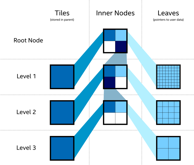
The data structure is a hierarchical regular grid at its core: Nodes are regular grids, and each grid cell may either store a constant value (this is called a tile), or child pointers. Nodes in VDB trees are wide: Nodes on the first level have a resolution of 32³ voxels, on the next level 16³, and on the leaf level 8³ voxels. All nodes on a given level have the same resolution. This makes it easy to find the node containing a coordinate using shift operations (see [1]). VDB leaf nodes are implicit in OSPRay / Open VKL: they are stored as pointers to user-provided data.

Topology of VDB volumes.

VDB volumes interpret input data as constant cells (which are then potentially filtered). This is in contrast to structuredRegular volumes, which have a vertex-centered interpretation.

The VDB implementation in OSPRay / Open VKL follows the following goals:

• Efficient data structure traversal on vector architectures.
• Enable the use of industry-standard .vdb files created through the OpenVDB library.
• Compatibility with OpenVDB on a leaf data level, so that .vdb file may be loaded with minimal overhead.

VDB volumes have the following parameters:

Type	Name	Description
int	maxSamplingDepth	do not descend further than to this depth during sampling, the maximum value and the default is 3
uint32[]	node.level	level on which each input node exists, may be 1, 2 or 3 (levels are counted from the root level = 0 down)
vec3i[]	node.origin	the node origin index (per input node)
OSPData[]	node.data	data arrays with the node data (per input node). Nodes that are tiles are expected to have single-item arrays. Leaf-nodes with grid data expected to have compact 3D arrays in zyx layout (z changes most quickly) with the correct number of voxels for the level. Only OSP_FLOAT is supported as field OSPDataType.
OSPData	nodesPackedDense	optionally provided instead of node.data, a single array of all dense node data in a contiguous zyx layout, provided in the same order as the corresponding node.* parameters
OSPData	nodesPackedTile	optionally provided instead of node.data, a single array of all tile node data in a contiguous layout, provided in the same order as the corresponding node.* parameters
uint32[]	node.format	for each input node, whether it is of format OSP_VOLUME_FORMAT_DENSE_ZYX (and thus stored in nodesPackedDense), or OSP_VOLUME_FORMAT_TILE (stored in nodesPackedTile)
uint	filter	filter used for reconstructing the field, default is OSP_VOLUME_FILTER_LINEAR, alternatively OSP_VOLUME_FILTER_NEAREST, or OSP_VOLUME_FILTER_CUBIC.
uint	gradientFilter	filter used for reconstructing the field during gradient computations, default same as filter
float	background	value that is used when sampling an undefined region outside the volume domain, default NaN

Configuration parameters for VDB volumes.

The nodesPackedDense and nodesPackedTile together with node.format parameters may be provided instead of node.data; this packed data layout may provide better performance.

1. Museth, K. VDB: High-Resolution Sparse Volumes with Dynamic Topology. ACM Transactions on Graphics 32(3), 2013. DOI: 10.1145/2487228.2487235

Particle Volume

Particle volumes consist of a set of points in space. Each point has a position, a radius, and a weight typically associated with an attribute. Particle volumes are created by passing the type string “particle” to ospNewVolume.

A radial basis function defines the contribution of that particle. Currently, we use the Gaussian radial basis function $$\phi(P) = w \exp\left(-\frac{(P - p)^2}{2 r^2}\right),$$ where $P$ is the particle position, $p$ is the sample position, $r$ is the radius and $w$ is the weight. At each sample, the scalar field value is then computed as the sum of each radial basis function $\phi$, for each particle that overlaps it.

The OSPRay / Open VKL implementation is similar to direct evaluation of samples in Reda et al. [2]. It uses an Embree-built BVH with a custom traversal, similar to the method in [1].

Type	Name	Default	Description
vec3f[]	particle.position		data array of particle positions
float[]	particle.radius		data array of particle radii
float[]	particle.weight	NULL	optional data array of particle weights, specifying the height of the kernel.
float	radiusSupportFactor	3.0	The multiplier of the particle radius required for support. Larger radii ensure smooth results at the cost of performance. In the Gaussian kernel, the radius is one standard deviation ($\sigma$), so a value of 3 corresponds to $3 \sigma$.
float	clampMaxCumulativeValue	0	The maximum cumulative value possible, set by user. All cumulative values will be clamped to this, and further traversal (RBF summation) of particle contributions will halt when this value is reached. A value of zero or less turns this off.
bool	estimateValueRanges	true	Enable heuristic estimation of value ranges which are used in internal acceleration structures as well as for determining the volume’s overall value range. When set to false, the user must specify clampMaxCumulativeValue, and all value ranges will be assumed [0–clampMaxCumulativeValue]. Disabling this switch may improve volume commit time, but will make volume rendering less efficient.

Configuration parameters for particle volumes.

1. A. Knoll, I. Wald, P. Navratil, A. Bowen, K. Reda, M.E., Papka, and K. Gaither, “RBF Volume Ray Casting on Multicore and Manycore CPUs”, 2014, Computer Graphics Forum, 33: 71–80. doi:10.1111/cgf.12363

2. K. Reda, A. Knoll, K. Nomura, M. E. Papka, A. E. Johnson and J. Leigh, “Visualizing large-scale atomistic simulations in ultra-resolution immersive environments”, 2013 IEEE Symposium on Large-Scale Data Analysis and Visualization (LDAV), Atlanta, GA, 2013, pp. 59–65.

Transfer Function

Transfer functions map the scalar values of volumes to color and opacity and thus they can be used to visually emphasize certain features of the volume. To create a new transfer function of given type type use

OSPTransferFunction ospNewTransferFunction(const char *type);

The returned handle can be assigned to a volumetric model (described below) as parameter “transferFunction” using ospSetObject.

One type of transfer function that is supported by OSPRay is the linear transfer function, which interpolates between given equidistant colors and opacities. It is create by passing the string “piecewiseLinear” to ospNewTransferFunction and it is controlled by these parameters:

Type	Name	Description
vec3f[]	color	data array of colors (linear RGB)
float[]	opacity	data array of opacities
box1f	value	domain (scalar range) this function maps from

Parameters accepted by the linear transfer function.

The arrays color and opacity can be of different length.

VolumetricModels

Volumes in OSPRay are given volume rendering appearance information through VolumetricModels. This decouples the physical representation of the volume (and possible acceleration structures it contains) to rendering-specific parameters (where more than one set may exist concurrently). To create a volume instance, call

OSPVolumetricModel ospNewVolumetricModel(OSPVolume);

The passed volume can be NULL as long as the volume to be used is passed as a parameter. If both a volume is specified on object creation and as a parameter, the parameter value is used. If the parameter value is later removed, the volume object passed on object creation is again used.

Type	Name	Default	Description
OSPVolume	volume		optional volume object this model references
OSPTransferFunction	transferFunction		transfer function to use
float	densityScale	1.0	makes volumes uniformly thinner or thicker
float	anisotropy	0.0	anisotropy of the (Henyey-Greenstein) phase function in [-1–1] (path tracer only), default to isotropic scattering
uint32	id	-1u	optional user ID, for framebuffer channel OSP_FB_ID_OBJECT

Parameters understood by VolumetricModel.

Geometries

Geometries in OSPRay are objects that describe intersectable surfaces. To create a new geometry object of given type type use

OSPGeometry ospNewGeometry(const char *type);

Note that in the current implementation geometries are limited to a maximum of 2³² primitives.

Mesh

A mesh consisting of either triangles or quads is created by calling ospNewGeometry with type string “mesh”. Once created, a mesh recognizes the following parameters:

Type	Name	Description
vec3f[]	vertex.position	data array of vertex positions, overridden by motion.* arrays
vec3f[]	normal	data array of face-varying normals, overridden by motion.* arrays
vec3f[]	vertex.normal	data array of vertex-varying normals, overridden by motion.* arrays
vec4f[] / vec3f[]	color	data array of face-varying colors (linear RGBA/RGB)
vec4f[] / vec3f[]	vertex.color	data array of vertex-varying colors (linear RGBA/RGB)
vec2f[]	texcoord	data array of face-varying texture coordinates
vec2f[]	vertex.texcoord	data array of vertex-varying texture coordinates
vec3ui[] / vec4ui[]	index	data array of (either triangle or quad) indices (into the vertex array(s))
bool	quadSoup	when no explicit index is given, indicates whether to assume a ‘soup’ of quads instead of triangles, default false
vec3f[][]	motion.vertex.position	data array of vertex position arrays (uniformly distributed keys for deformation motion blur)
vec3f[][]	motion.normal	data array of face-varying normal arrays (uniformly distributed keys for deformation motion blur)
vec3f[][]	motion.vertex.normal	data array of vertex-varying normal arrays (uniformly distributed keys for deformation motion blur)
box1f	time	time associated with first and last key in motion.* arrays (for deformation motion blur), default [0, 1]

Parameters defining a mesh geometry.

The data type of index arrays differentiates between the underlying geometry, triangles are used for a index with vec3ui type and quads for vec4ui type. Quads are internally handled as a pair of two triangles, thus mixing triangles and quads is supported by encoding some triangle as a quad with the last two vertex indices being identical (w=z).

The vertex.position array is mandatory to create a valid mesh.

The index array is optional. If none is provided, a ‘triangle soup’ is assumed, i.e., each three consecutive vertices form one triangle; unless the boolean quadSoup is set to true, then a ‘quad soup’ is assumed i.e., each four subsequent vertices form one quad. If the size of the vertex.position array is not a multiple of three for triangles or four for quads, the remainder vertices are ignored.

Subdivision

A mesh consisting of subdivision surfaces, created by specifying a geometry of type “subdivision”. Once created, a subdivision recognizes the following parameters:

Type	Name	Description
vec3f[]	vertex.position	data array of vertex positions
vec4f[]	color	optional data array of face-varying colors (linear RGBA)
vec4f[]	vertex.color	optional data array of vertex-varying colors (linear RGBA)
vec2f[]	texcoord	optional data array of vertex-varying texture coordinates
vec2f[]	vertex.texcoord	optional data array of vertex-varying texture coordinates
float	level	global level of tessellation, default 5
uint[]	index	data array of indices (into the vertex array(s))
float[]	index.level	optional data array of per-edge levels of tessellation, overrides global level
uint[]	face	optional data array holding the number of indices/edges (3 to 15) per face, defaults to 4 (a pure quad mesh)
vec2i[]	edgeCrease.index	optional data array of edge crease indices
float[]	edgeCrease.weight	optional data array of edge crease weights
uint[]	vertexCrease.index	optional data array of vertex crease indices
float[]	vertexCrease.weight	optional data array of vertex crease weights
uint	mode	OSPSubdivisionMode subdivision edge boundary mode, supported modes are:
		OSP_SUBDIVISION_NO_BOUNDARY
		OSP_SUBDIVISION_SMOOTH_BOUNDARY (default)
		OSP_SUBDIVISION_PIN_CORNERS
		OSP_SUBDIVISION_PIN_BOUNDARY
		OSP_SUBDIVISION_PIN_ALL

Parameters defining a Subdivision geometry.

The vertex and index arrays are mandatory to create a valid subdivision surface. If no face array is present then a pure quad mesh is assumed (the number of indices must be a multiple of 4). Optionally supported are edge and vertex creases.

Spheres

A geometry consisting of individual spheres, each of which can have an own radius, is created by calling ospNewGeometry with type string “sphere”. The spheres will not be tessellated but rendered procedurally and are thus perfectly round. To allow a variety of sphere representations in the application this geometry allows a flexible way of specifying the data of center position and radius within a data array:

Type	Name	Default	Description
vec3f[]	sphere.position		data array of center positions
float[]	sphere.radius	NULL	optional data array of the per-sphere radius
vec3f[]	sphere.normal	NULL	optional data array of normals (only for “oriented disc”)
vec2f[]	sphere.texcoord	NULL	optional data array of texture coordinates (constant per sphere)
float	radius	0.01	default radius for all spheres (if sphere.radius is not set)
uint	type		OSPSphereType for rendering the sphere. Supported types are:
			OSP_SPHERE (default)
			OSP_DISC
			OSP_ORIENTED_DISC

Parameters defining a spheres geometry.

Curves

A geometry consisting of multiple curves is created by calling ospNewGeometry with type string “curve”. The parameters defining this geometry are listed in the table below.

Type	Name	Description
vec4f[]	vertex.position_radius	data array of vertex position and per-vertex radius
vec2f[]	vertex.texcoord	data array of per-vertex texture coordinates
vec4f[]	vertex.color	data array of corresponding vertex colors (linear RGBA)
vec3f[]	vertex.normal	data array of curve normals (only for “ribbon” curves)
vec4f[]	vertex.tangent	data array of curve tangents (only for “hermite” curves)
uint32[]	index	data array of indices to the first vertex or tangent of a curve segment
uint	type	OSPCurveType for rendering the curve. Supported types are:
		OSP_FLAT
		OSP_ROUND
		OSP_RIBBON
		OSP_DISJOINT
uint	basis	OSPCurveBasis for defining the curve. Supported bases are:
		OSP_LINEAR
		OSP_BEZIER
		OSP_BSPLINE
		OSP_HERMITE
		OSP_CATMULL_ROM

Parameters defining a curves geometry.

Positions in vertex.position_radius parameter supports per-vertex varying radii with data type vec4f[] and instantiate Embree curves internally for the relevant type/basis mapping.

The following section describes the properties of different curve basis’ and how they use the data provided in data buffers:

OSP_LINEAR
The indices point to the first of 2 consecutive control points in the vertex buffer. The first control point is the start and the second control point the end of the line segment. The curve goes through all control points listed in the vertex buffer.

OSP_BEZIER
The indices point to the first of 4 consecutive control points in the vertex buffer. The first control point represents the start point of the curve, and the 4th control point the end point of the curve. The Bézier basis is interpolating, thus the curve does go exactly through the first and fourth control vertex.

OSP_BSPLINE
The indices point to the first of 4 consecutive control points in the vertex buffer. This basis is not interpolating, thus the curve does in general not go through any of the control points directly. Using this basis, 3 control points can be shared for two continuous neighboring curve segments, e.g., the curves $(p0, p1, p2, p3)$ and $(p1, p2, p3, p4)$ are C1 continuous. This feature make this basis a good choice to construct continuous multi-segment curves, as memory consumption can be kept minimal.

OSP_HERMITE
It is necessary to have both vertex buffer and tangent buffer for using this basis. The indices point to the first of 2 consecutive points in the vertex buffer, and the first of 2 consecutive tangents in the tangent buffer. This basis is interpolating, thus does exactly go through the first and second control point, and the first order derivative at the begin and end matches exactly the value specified in the tangent buffer. When connecting two segments continuously, the end point and tangent of the previous segment can be shared.

OSP_CATMULL_ROM
The indices point to the first of 4 consecutive control points in the vertex buffer. If $(p0, p1, p2, p3)$ represent the points then this basis goes through $p1$ and $p2$, with tangents as $(p2-p0)/2$ and $(p3-p1)/2$.

The following section describes the properties of different curve types’ and how they define the geometry of a curve:

OSP_FLAT
This type enables faster rendering as the curve is rendered as a connected sequence of ray facing quads.

OSP_ROUND
This type enables rendering a real geometric surface for the curve which allows closeup views. This mode renders a sweep surface by sweeping a varying radius circle tangential along the curve.

OSP_RIBBON
The type enables normal orientation of the curve and requires a normal buffer be specified along with vertex buffer. The curve is rendered as a flat band whose center approximately follows the provided vertex buffer and whose normal orientation approximately follows the provided normal buffer. Not supported for basis OSP_LINEAR.

OSP_DISJOINT
Only supported for basis OSP_LINEAR; the segments are open and not connected at the joints, i.e., the curve segments are either individual cones or cylinders.

Boxes

OSPRay can directly render axis-aligned bounding boxes without the need to convert them to quads or triangles. To do so create a boxes geometry by calling ospNewGeometry with type string “box”.

Type	Name	Description
box3f[]	box	data array of boxes

Parameters defining a boxes geometry.

Planes

OSPRay can directly render planes defined by plane equation coefficients in its implicit form $ax + by + cz + d = 0$. By default planes are infinite but their extents can be limited by defining optional bounding boxes. A planes geometry can be created by calling ospNewGeometry with type string “plane”.

Type	Name	Description
vec4f[]	plane.coefficients	data array of plane coefficients $(a, b, c, d)$
box3f[]	plane.bounds	optional data array of bounding boxes

Parameters defining a planes geometry.

Isosurfaces

OSPRay can directly render multiple isosurfaces of a volume without first tessellating them. To do so create an isosurfaces geometry by calling ospNewGeometry with type string “isosurface”. The appearance information of the surfaces is set through the Geometric Model. Per-isosurface colors can be set by passing per-primitive colors to the Geometric Model, in order of the isosurface array.

Type	Name	Description
float	isovalue	single isovalues
float[]	isovalue	data array of isovalues
OSPVolume	volume	handle of the Volume to be isosurfaced

Parameters defining an isosurfaces geometry.

GeometricModels

Geometries are matched with surface appearance information through GeometricModels. These take a geometry, which defines the surface representation, and applies either full-object or per-primitive color and material information. To create a geometric model, call

OSPGeometricModel ospNewGeometricModel(OSPGeometry);

The passed geometry can be NULL as long as the geometry to be used is passed as a parameter. If both a geometry is specified on object creation and as a parameter, the parameter value is used. If the parameter value is later removed, the geometry object passed on object creation is again used.

Color and material are fetched with the primitive ID of the hit (clamped to the valid range, thus a single color or material is fine), or mapped first via the index array (if present). All parameters are optional, however, some renderers (notably the path tracer) require a material to be set. Materials are either handles of OSPMaterial, or indices into the material array on the renderer, which allows to build a world which can be used by different types of renderers.

An invertNormals flag allows to invert (shading) normal vectors of the rendered geometry. That is particularly useful for clipping. By changing normal vectors orientation one can control whether inside or outside of the clipping geometry is being removed. For example, a clipping geometry with normals oriented outside clips everything what’s inside.

Type	Name	Description
OSPGeometry	geometry	optional geometry object this model references
OSPMaterial / OSPMaterial[] / uint32 / uint32[]	material	optional (data array of per-primitive) material, may be an index into the material parameter on the renderer (if it exists)
vec4f / vec4f[]	color	optional (data array of per-primitive) color assigned to the geometry (linear RGBA)
uint8[]	index	optional data array of per-primitive indices into color and material
bool	invertNormals	inverts all shading normals (Ns), default false
uint32	id	optional user ID, for framebuffer channel OSP_FB_ID_OBJECT, default -1u

Parameters understood by GeometricModel.

Lights

To create a new light source of given type type use

OSPLight ospNewLight(const char *type);

All light sources accept the following parameters:

Type	Name	Default	Description
vec3f	color	white	color of the light (linear RGB)
float	intensity	1	intensity of the light (a factor)
uint	intensityQuantity		OSPIntensityQuantity to set the radiometric quantity represented by intensity. The default value depends on the light source.
bool	visible	true	whether the light can be directly seen

Parameters accepted by all lights.

In OSPRay the intensity parameter of a light source can correspond to different types of radiometric quantities. The type of the value represented by a light’s intensity parameter is set using intensityQuantity, which accepts values from the enum type OSPIntensityQuantity. The supported types of OSPIntensityQuantity differ between the different light sources (see documentation of each specific light source).

Name	Description
OSP_INTENSITY_QUANTITY_POWER	the overall amount of light energy emitted by the light source into the scene, unit is W
OSP_INTENSITY_QUANTITY_INTENSITY	the overall amount of light emitted by the light in a given direction, unit is W/sr
OSP_INTENSITY_QUANTITY_RADIANCE	the amount of light emitted by a point on the light source in a given direction, unit is W/sr/m2
OSP_INTENSITY_QUANTITY_IRRADIANCE	the amount of light arriving at a surface point, assuming the light is oriented towards to the surface, unit is W/m2
OSP_INTENSITY_QUANTITY_SCALE	a linear scaling factor for light sources with a built-in quantity (e.g., HDRI, or sunSky, or when using intensityDistribution).

Types of radiometric quantities used to interpret a light’s intensity parameter.

Photometric Lights

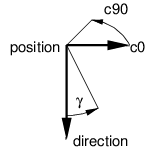
Measured light sources (IES, EULUMDAT, …) are supported by the sphere, spot, and quad lights when setting an intensityDistribution data array to modulate the intensity per direction. The mapping is using the C-γ coordinate system (see also below figure): the values of the first (or only) dimension of intensityDistribution are uniformly mapped to γ in [0–π]; the first intensity value to 0, the last value to π, thus at least two values need to be present.

If the array has a second dimension then the intensities are not rotational symmetric around the main direction (where angle γ is zero), but are accordingly mapped to the C-halfplanes in [0–2π]; the first “row” of values to 0 and 2π, the other rows such that they have uniform distance to its neighbors. The orientation of the C0-plane is specified via c0.

Type	Name	Description
float[]	intensityDistribution	luminous intensity distribution for photometric lights; can be 2D for asymmetric illumination; values are assumed to be uniformly distributed
vec3f	c0	orientation, i.e., direction of the C0-(half)plane (only needed if illumination via intensityDistribution is asymmetric)

Special parameters for photometric lights.

When using an intensityDistribution then the default and only valid value for intensityQuantity is OSP_INTENSITY_QUANTITY_SCALE.

The following light types are supported by most OSPRay renderers.

Directional Light / Distant Light

The distant light (or traditionally the directional light) is thought to be far away (outside of the scene), thus its light arrives (almost) as parallel rays. It is created by passing the type string “distant” to ospNewLight. The distant light supports OSP_INTENSITY_QUANTITY_RADIANCE and OSP_INTENSITY_QUANTITY_IRRADIANCE (default) as intensityQuantity parameter value. In addition to the general parameters understood by all lights the distant light supports the following special parameters:

Type	Name	Default	Description
vec3f	direction	$(0, 0, 1)$	main emission direction of the distant light
float	angularDiameter	0	apparent size (angle in degree) of the light

Special parameters accepted by the distant light.

Setting the angular diameter to a value greater than zero will result in soft shadows when the renderer uses stochastic sampling (like the path tracer). For instance, the apparent size of the sun is about 0.53°.

Point Light / Sphere Light

The sphere light (or the special case point light) is a light emitting uniformly in all directions from the surface toward the outside. It does not emit any light toward the inside of the sphere. It is created by passing the type string “sphere” to ospNewLight. The point light supports only OSP_INTENSITY_QUANTITY_SCALE when intensityDistribution is set, or otherwise OSP_INTENSITY_QUANTITY_POWER, OSP_INTENSITY_QUANTITY_INTENSITY (then default) and OSP_INTENSITY_QUANTITY_RADIANCE as intensityQuantity parameter value. In addition to the general parameters understood by all lights and the photometric parameters the sphere light supports the following special parameters:

Type	Name	Default	Description
vec3f	position	$(0, 0, 0)$	the center of the sphere light
float	radius	0	the size of the sphere light
vec3f	direction	$(0, 0, 1)$	main orientation of intensityDistribution

Special parameters accepted by the sphere light.

Setting the radius to a value greater than zero will result in soft shadows when the renderer uses stochastic sampling (like the path tracer).

Spotlight / Ring Light

The spotlight is a light emitting into a cone of directions. It is created by passing the type string “spot” to ospNewLight. The spotlight supports only OSP_INTENSITY_QUANTITY_SCALE when intensityDistribution is set, or otherwise OSP_INTENSITY_QUANTITY_POWER, OSP_INTENSITY_QUANTITY_INTENSITY (then default) and OSP_INTENSITY_QUANTITY_RADIANCE as intensityQuantity parameter value. In addition to the general parameters understood by all lights and the photometric parameters the spotlight supports the special parameters listed in the table.

Type	Name	Default	Description
vec3f	position	$(0, 0, 0)$	the center of the spotlight
vec3f	direction	$(0, 0, 1)$	main emission direction of the spot
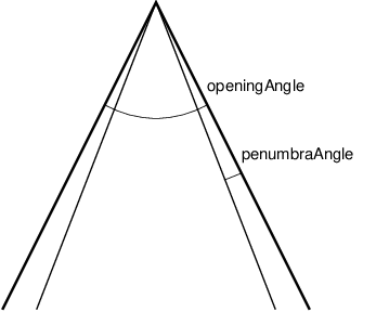
float	openingAngle	180	full opening angle (in degree) of the spot; outside of this cone is no illumination
float	penumbraAngle	5	size (angle in degree) of the “penumbra”, the region between the rim (of the illumination cone) and full intensity of the spot; should be smaller than half of openingAngle
float	radius	0	the size of the spotlight, the radius of a disk with normal direction
float	innerRadius	0	in combination with radius turns the disk into a ring

Special parameters accepted by the spotlight.

Setting the radius to a value greater than zero will result in soft shadows when the renderer uses stochastic sampling (like the path tracer). Additionally setting the inner radius will result in a ring instead of a disk emitting the light.

Quad Light

The quad⁴ light is a planar, procedural area light source emitting uniformly on one side into the half-space. It is created by passing the type string “quad” to ospNewLight. The quad light supports only OSP_INTENSITY_QUANTITY_SCALE when intensityDistribution is set, or otherwise OSP_INTENSITY_QUANTITY_POWER, OSP_INTENSITY_QUANTITY_INTENSITY and OSP_INTENSITY_QUANTITY_RADIANCE (then default) as intensityQuantity parameter. In addition to the general parameters understood by all lights and the photometric parameters the quad light supports the following special parameters:

Type	Name	Default	Description
vec3f	position	$(0, 0, 0)$	position of one vertex of the quad light
vec3f	edge1	$(1, 0, 0)$	vector to one adjacent vertex
vec3f	edge2	$(0, 1, 0)$	vector to the other adjacent vertex

Special parameters accepted by the quad light.

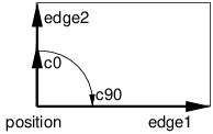
The emission side is determined by the cross product of edge1×edge2. which is also the main emission direction for intensityDistribution. Note that only renderers that use stochastic sampling (like the path tracer) will compute soft shadows from the quad light. Other renderers will just sample the center of the quad light, which results in hard shadows.

Cylinder Light

The cylinder light is a cylinderical, procedural area light source emitting uniformly outwardly into the space beyond the boundary. It is created by passing the type string “cylinder” to ospNewLight. The cylinder light supports OSP_INTENSITY_QUANTITY_POWER, OSP_INTENSITY_QUANTITY_INTENSITY and OSP_INTENSITY_QUANTITY_RADIANCE (default) as intensityQuantity parameter. In addition to the general parameters understood by all lights the cylinder light supports the following special parameters:

Type	Name	Default	Description
vec3f	position0	$(0, 0, 0)$	position of the start of the cylinder
vec3f	position1	$(0, 0, 1)$	position of the end of the cylinder
float	radius	1	radius of the cylinder

Special parameters accepted by the cylinder light.

Note that only renderers that use stochastic sampling (like the path tracer) will compute soft shadows from the cylinder light. Other renderers will just sample the closest point on the cylinder light, which results in hard shadows.

HDRI Light

The HDRI light is a textured light source surrounding the scene and illuminating it from infinity. It is created by passing the type string “hdri” to ospNewLight. The values of the HDRI correspond to radiance and therefore the HDRI light only accepts OSP_INTENSITY_QUANTITY_SCALE as intensityQuantity parameter value. In addition to the general parameters the HDRI light supports the following special parameters:

Type	Name	Default	Description
vec3f	up	$(0, 1, 0)$	up direction of the light
vec3f	direction	$(0, 0, 1)$	direction to which the center of the texture will be mapped to (analog to panoramic camera)
OSPTexture	map		environment map in latitude / longitude format

Special parameters accepted by the HDRI light.

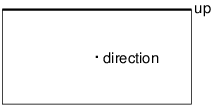
Note that the SciVis renderer only shows the HDRI light in the background (like an environment map) without computing illumination of the scene.

Ambient Light

The ambient light surrounds the scene and illuminates it from infinity with constant radiance (determined by combining the parameters color and intensity). It is created by passing the type string “ambient” to ospNewLight. The ambient light supports OSP_INTENSITY_QUANTITY_RADIANCE and OSP_INTENSITY_QUANTITY_IRRADIANCE (default) as intensityQuantity parameter value.

Note that the SciVis renderer uses ambient lights to control the color and intensity of the computed ambient occlusion (AO).

Sun-Sky Light

The sun-sky light is a combination of a distant light for the sun and a procedural hdri light for the sky. It is created by passing the type string “sunSky” to ospNewLight. The sun-sky light surrounds the scene and illuminates it from infinity and can be used for rendering outdoor scenes. The radiance values are calculated using the Hošek-Wilkie sky model and solar radiance function. The underlying model of the sun-sky light returns radiance values and therefore the light only accepts OSP_INTENSITY_QUANTITY_SCALE as intensityQuantity parameter value. To rescale the returned radiance of the sky model the default value for the intensity parameter is set to 0.025. In addition to the general parameters the following special parameters are supported:

Type	Name	Default	Description
vec3f	up	$(0, 1, 0)$	zenith of sky
vec3f	direction	$(0, -1, 0)$	main emission direction of the sun
float	turbidity	3	atmospheric turbidity due to particles, in [1–10]
float	albedo	0.3	ground reflectance, in [0–1]
float	horizonExtension	0.01	extend the sky dome by stretching the horizon, fraction of the lower hemisphere to cover, in [0–1]

Special parameters accepted by the sunSky light.

The lowest elevation for the sun is restricted to the horizon.

Note that the SciVis renderer only computes illumination from the sun (yet the sky is still shown in the background, like an environment map).

Emissive Objects

The path tracer will consider illumination by geometries which have a light emitting material assigned (for example the Luminous or Principled material).

Materials

Materials describe how light interacts with surfaces, they give objects their distinctive look. To create a new material of given type type call

OSPMaterial ospNewMaterial(const char *material_type);

The returned handle can then be used to assign the material to a given geometry with

void ospSetObject(OSPGeometricModel, "material", OSPMaterial);

OBJ Material

The OBJ material is the workhorse material supported by both the SciVis renderer and the path tracer (the Ambient Occlusion renderer only uses the kd and d parameter). It offers widely used common properties like diffuse and specular reflection and is based on the MTL material format of Lightwave’s OBJ scene files. To create an OBJ material pass the type string “obj” to ospNewMaterial. Its main parameters are

Type	Name	Default	Description
vec3f	kd	white 0.8	diffuse color (linear RGB)
vec3f	ks	black	specular color (linear RGB)
float	ns	10	shininess (Phong exponent), usually in [2–104]
float	d	opaque	opacity
vec3f	tf	black	transparency filter color (linear RGB)
OSPTexture	map_bump	NULL	normal map

Main parameters of the OBJ material.

In particular when using the path tracer it is important to adhere to the principle of energy conservation, i.e., that the amount of light reflected by a surface is not larger than the light arriving. Therefore the path tracer issues a warning and renormalizes the color parameters if the sum of kd, ks, and tf is larger than one in any color channel. Similarly important to mention is that almost all materials of the real world reflect at most only about 80% of the incoming light. So even for a white sheet of paper or white wall paint do better not set kd larger than 0.8; otherwise rendering times are unnecessary long and the contrast in the final images is low (for example, the corners of a white room would hardly be discernible, as can be seen in the figure below).

Comparison of diffuse rooms with 100% reflecting white paint (left) and realistic 80% reflecting white paint (right), which leads to higher overall contrast. Note that exposure has been adjusted to achieve similar brightness levels.

If present, the color component of geometries is also used for the diffuse color kd and the alpha component is also used for the opacity d.

Normal mapping can simulate small geometric features via the texture map_bump. The normals $n$ in the normal map are with respect to the local tangential shading coordinate system and are encoded as $½(n+1)$, thus a texel $(0.5, 0.5, 1)$⁵ represents the unperturbed shading normal $(0, 0, 1)$. Because of this encoding an sRGB gamma texture format is ignored and normals are always fetched as linear from a normal map. Note that the orientation of normal maps is important for a visually consistent look: by convention OSPRay uses a coordinate system with the origin in the lower left corner; thus a convexity will look green toward the top of the texture image (see also the example image of a normal map). If this is not the case flip the normal map vertically or invert its green channel.

Normal map representing an exalted square pyramidal frustum.

Note that tf colored transparency is implemented in the SciVis and the path tracer but normal mapping with map_bump is currently supported in the path tracer only.

All parameters (except tf) can be textured by passing a texture handle, prefixed with “map_”. The fetched texels are multiplied by the respective parameter value. If only the texture is given (but not the corresponding parameter), only the texture is used (the default value of the parameter is not multiplied). The color textures map_kd and map_ks are typically in one of the sRGB gamma encoded formats, whereas textures map_ns and map_d are usually in a linear format (and only the first component is used). Additionally, all textures support texture transformations.

Rendering of a OBJ material with wood textures.

Principled

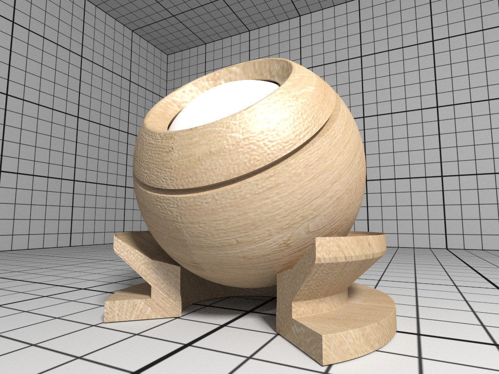
The Principled material is the most complex material offered by the path tracer, which is capable of producing a wide variety of materials (e.g., plastic, metal, wood, glass) by combining multiple different layers and lobes. It uses the GGX microfacet distribution with approximate multiple scattering for dielectrics and metals, uses the Oren-Nayar model for diffuse reflection, and is energy conserving. To create a Principled material, pass the type string “principled” to ospNewMaterial. Its parameters are listed in the table below.

Type	Name	Default	Description
vec3f	baseColor	white 0.8	base reflectivity (diffuse and/or metallic, linear RGB)
vec3f	edgeColor	white	edge tint (metallic only, linear RGB)
float	metallic	0	mix between dielectric (diffuse and/or specular) and metallic (specular only with complex IOR) in [0–1]
float	diffuse	1	diffuse reflection weight in [0–1]
float	specular	1	specular reflection/transmission weight in [0–1]
float	ior	1	dielectric index of refraction
float	transmission	0	specular transmission weight in [0–1]
vec3f	transmissionColor	white	attenuated color due to transmission (Beer’s law, linear RGB)
float	transmissionDepth	1	distance at which color attenuation is equal to transmissionColor
float	roughness	0	diffuse and specular roughness in [0–1], 0 is perfectly smooth
float	anisotropy	0	amount of specular anisotropy in [0–1]
float	rotation	0	rotation of the direction of anisotropy in [0–1], 1 is going full circle
float	normal	1	default normal map/scale for all layers
float	baseNormal	1	base normal map/scale (overrides default normal)
bool	thin	false	flag specifying whether the material is thin or solid
float	thickness	1	thickness of the material (thin only), affects the amount of color attenuation due to specular transmission
float	backlight	0	amount of diffuse transmission (thin only) in [0–2], 1 is 50% reflection and 50% transmission, 2 is transmission only
float	coat	0	clear coat layer weight in [0–1]
float	coatIor	1.5	clear coat index of refraction
vec3f	coatColor	white	clear coat color tint (linear RGB)
float	coatThickness	1	clear coat thickness, affects the amount of color attenuation
float	coatRoughness	0	clear coat roughness in [0–1], 0 is perfectly smooth
float	coatNormal	1	clear coat normal map/scale (overrides default normal)
float	sheen	0	sheen layer weight in [0–1]
vec3f	sheenColor	white	sheen color tint (linear RGB)
float	sheenTint	0	how much sheen is tinted from sheenColor toward baseColor
float	sheenRoughness	0.2	sheen roughness in [0–1], 0 is perfectly smooth
float	opacity	1	cut-out opacity/transparency, 1 is fully opaque
vec3f	emissiveColor	black	color (and intensity) of the emitted light

Parameters of the Principled material.

All parameters can be textured by passing a texture handle, prefixed with “map_” (e.g., “map_baseColor”). texture transformations are supported as well.

Rendering of a Principled coated brushed metal material with textured anisotropic rotation and a dust layer (sheen) on top.

CarPaint

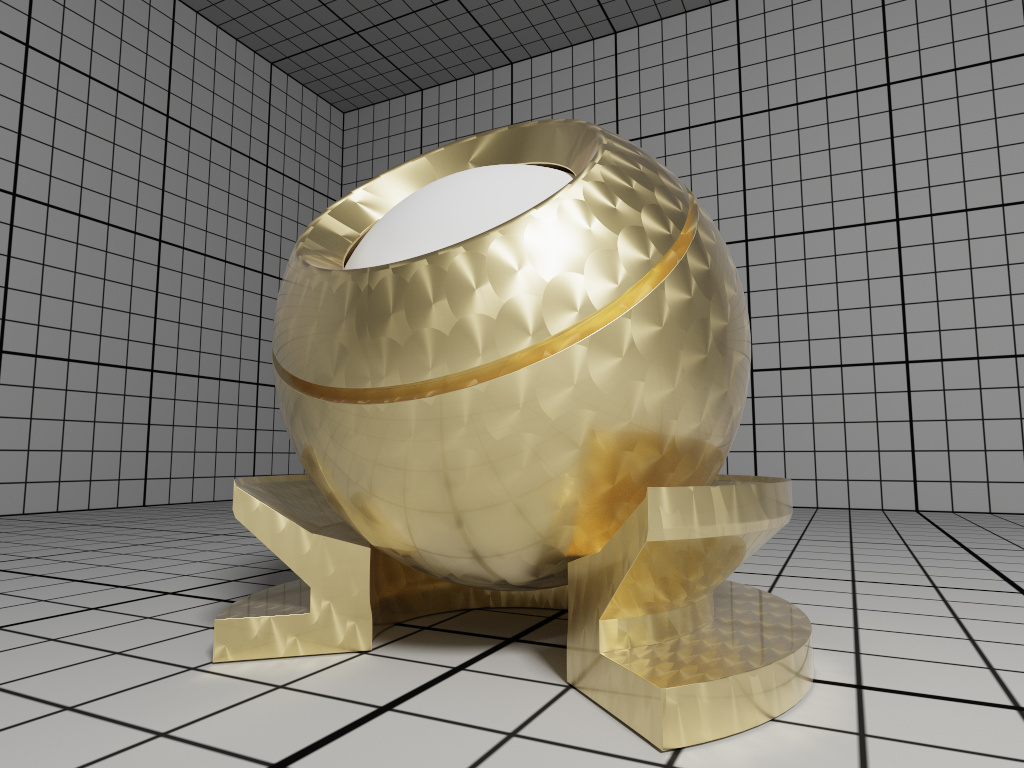
The CarPaint material is a specialized version of the Principled material for rendering different types of car paints. To create a CarPaint material, pass the type string “carPaint” to ospNewMaterial. Its parameters are listed in the table below.

Type	Name	Default	Description
vec3f	baseColor	white 0.8	diffuse base reflectivity (linear RGB)
float	roughness	0	diffuse roughness in [0–1], 0 is perfectly smooth
float	normal	1	normal map/scale
vec3f	flakeColor	Aluminium	color of metallic flakes (linear RGB)
float	flakeDensity	0	density of metallic flakes in [0–1], 0 disables flakes, 1 fully covers the surface with flakes
float	flakeScale	100	scale of the flake structure, higher values increase the amount of flakes
float	flakeSpread	0.3	flake spread in [0–1]
float	flakeJitter	0.75	flake randomness in [0–1]
float	flakeRoughness	0.3	flake roughness in [0–1], 0 is perfectly smooth
float	coat	1	clear coat layer weight in [0–1]
float	coatIor	1.5	clear coat index of refraction
vec3f	coatColor	white	clear coat color tint (linear RGB)
float	coatThickness	1	clear coat thickness, affects the amount of color attenuation
float	coatRoughness	0	clear coat roughness in [0–1], 0 is perfectly smooth
float	coatNormal	1	clear coat normal map/scale
vec3f	flipflopColor	white	reflectivity of coated flakes at grazing angle, used together with coatColor produces a pearlescent paint (linear RGB)
float	flipflopFalloff	1	flip flop color falloff, 1 disables the flip flop effect

Parameters of the CarPaint material.

All parameters can be textured by passing a texture handle, prefixed with “map_” (e.g., “map_baseColor”). texture transformations are supported as well.

Rendering of a pearlescent CarPaint material.

Metal

The path tracer offers a physical metal, supporting changing roughness and realistic color shifts at edges. To create a Metal material pass the type string “metal” to ospNewMaterial. Its parameters are

Type	Name	Default	Description
vec3f[]	ior	Aluminium	data array of spectral samples of complex refractive index, each entry in the form (wavelength, eta, k), ordered by wavelength (which is in nm)
vec3f	eta		RGB complex refractive index, real part
vec3f	k		RGB complex refractive index, imaginary part
float	roughness	0.1	roughness in [0–1], 0 is perfect mirror

Parameters of the Metal material.

The main appearance (mostly the color) of the Metal material is controlled by the physical parameters eta and k, the wavelength-dependent, complex index of refraction. These coefficients are quite counter-intuitive but can be found in published measurements. For accuracy the index of refraction can be given as an array of spectral samples in ior, each sample a triplet of wavelength (in nm), eta, and k, ordered monotonically increasing by wavelength; OSPRay will then calculate the Fresnel in the spectral domain. Alternatively, eta and k can also be specified as approximated RGB coefficients; some examples are given in below table.

Metal	eta	k
Ag, Silver	(0.051, 0.043, 0.041)	(5.3, 3.6, 2.3)
Al, Aluminium	(1.5, 0.98, 0.6)	(7.6, 6.6, 5.4)
Au, Gold	(0.07, 0.37, 1.5)	(3.7, 2.3, 1.7)
Cr, Chromium	(3.2, 3.1, 2.3)	(3.3, 3.3, 3.1)
Cu, Copper	(0.1, 0.8, 1.1)	(3.5, 2.5, 2.4)

Index of refraction of selected metals as approximated RGB coefficients, based on data from https://refractiveindex.info/.

The roughness parameter controls the variation of microfacets and thus how polished the metal will look. The roughness can be modified by a texture map_roughness (texture transformations are supported as well) to create notable edging effects.

Rendering of golden Metal material with textured roughness.

Alloy

The path tracer offers an alloy material, which behaves similar to Metal, but allows for more intuitive and flexible control of the color. To create an Alloy material pass the type string “alloy” to ospNewMaterial. Its parameters are

Type	Name	Default	Description
vec3f	color	white 0.9	reflectivity at normal incidence (0 degree, linear RGB)
vec3f	edgeColor	white	reflectivity at grazing angle (90 degree, linear RGB)
float	roughness	0.1	roughness, in [0–1], 0 is perfect mirror

Parameters of the Alloy material.

The main appearance of the Alloy material is controlled by the parameter color, while edgeColor influences the tint of reflections when seen at grazing angles (for real metals this is always 100% white). If present, the color component of geometries is also used for reflectivity at normal incidence color. As in Metal the roughness parameter controls the variation of microfacets and thus how polished the alloy will look. All parameters can be textured by passing a texture handle, prefixed with “map_”; texture transformations are supported as well.

Rendering of a fictional Alloy material with textured color.

Glass

The path tracer offers a realistic a glass material, supporting refraction and volumetric attenuation (i.e., the transparency color varies with the geometric thickness). To create a Glass material pass the type string “glass” to ospNewMaterial. Its parameters are

Type	Name	Default	Description
float	eta	1.5	index of refraction
vec3f	attenuationColor	white	resulting color due to attenuation (linear RGB)
float	attenuationDistance	1	distance affecting attenuation

Parameters of the Glass material.

For convenience, the rather counter-intuitive physical attenuation coefficients will be calculated from the user inputs in such a way, that the attenuationColor will be the result when white light traveled through a glass of thickness attenuationDistance.

Rendering of a Glass material with orange attenuation.

ThinGlass

The path tracer offers a thin glass material useful for objects with just a single surface, most prominently windows. It models a thin, transparent slab, i.e., it behaves as if a second, virtual surface is parallel to the real geometric surface. The implementation accounts for multiple internal reflections between the interfaces (including attenuation), but neglects parallax effects due to its (virtual) thickness. To create a such a thin glass material pass the type string “thinGlass” to ospNewMaterial. Its parameters are

Type	Name	Default	Description
float	eta	1.5	index of refraction
vec3f	attenuationColor	white	resulting color due to attenuation (linear RGB)
float	attenuationDistance	1	distance affecting attenuation
float	thickness	1	virtual thickness

Parameters of the ThinGlass material.

For convenience the attenuation is controlled the same way as with the Glass material. Additionally, the color due to attenuation can be modulated with a texture map_attenuationColor (texture transformations are supported as well). If present, the color component of geometries is also used for the attenuation color. The thickness parameter sets the (virtual) thickness and allows for easy exchange of parameters with the (real) Glass material; internally just the ratio between attenuationDistance and thickness is used to calculate the resulting attenuation and thus the material appearance.

Rendering of a ThinGlass material with red attenuation.

Example image of a colored window made with textured attenuation of the ThinGlass material.

MetallicPaint

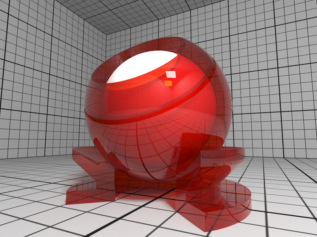
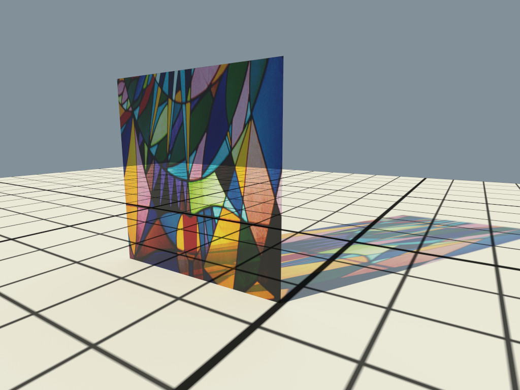
The path tracer offers a metallic paint material, consisting of a base coat with optional flakes and a clear coat. To create a MetallicPaint material pass the type string “metallicPaint” to ospNewMaterial. Its parameters are listed in the table below.

Type	Name	Default	Description
vec3f	baseColor	white 0.8	color of base coat (linear RGB)
float	flakeAmount	0.3	amount of flakes, in [0–1]
vec3f	flakeColor	Aluminium	color of metallic flakes (linear RGB)
float	flakeSpread	0.5	spread of flakes, in [0–1]
float	eta	1.5	index of refraction of clear coat

Parameters of the MetallicPaint material.

The color of the base coat baseColor can be textured by a texture map_baseColor, which also supports texture transformations. If present, the color component of geometries is also used for the color of the base coat. Parameter flakeAmount controls the proportion of flakes in the base coat, so when setting it to 1 the baseColor will not be visible. The shininess of the metallic component is governed by flakeSpread, which controls the variation of the orientation of the flakes, similar to the roughness parameter of Metal. Note that the effect of the metallic flakes is currently only computed on average, thus individual flakes are not visible.

Rendering of a MetallicPaint material.

Luminous

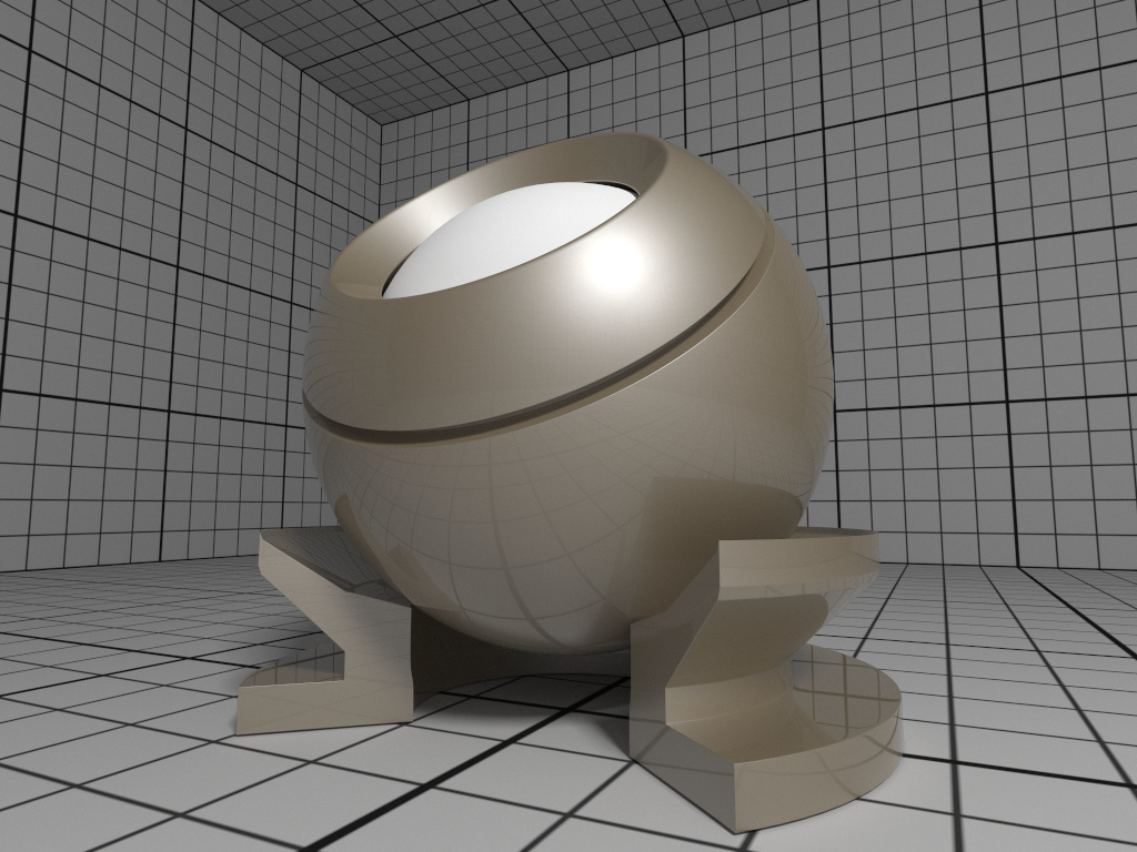
The path tracer supports the Luminous material which emits light uniformly in all directions and which can thus be used to turn any geometric object into a light source. It is created by passing the type string “luminous” to ospNewMaterial. The amount of constant radiance that is emitted is determined by combining the general parameters of lights: color and intensity (which essentially means that parameter intensityQuantity is not needed because it is always OSP_INTENSITY_QUANTITY_RADIANCE).

Type	Name	Default	Description
vec3f	color	white	color of the emitted light (linear RGB)
float	intensity	1	intensity of the light (a factor)
float	transparency	1	material transparency

Parameters accepted by the Luminous material.

The emission can be textured by passing a map_color texture handle, texture transformations are supported as well.

Rendering of a yellow Luminous material.

Texture

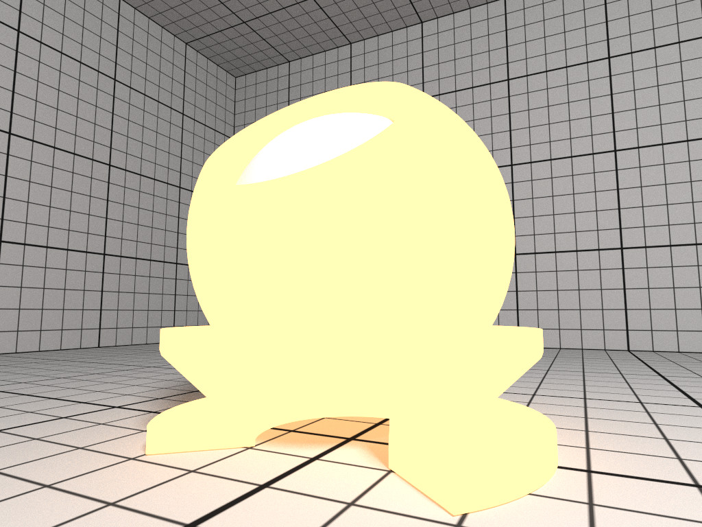
OSPRay currently implements two texture types (texture2d and volume) and is open for extension to other types by applications. More types may be added in future releases.

To create a new texture use

OSPTexture ospNewTexture(const char *type);

Texture2D

The texture2d texture type implements an image-based texture, where its parameters are as follows

Type	Name	Description
uint	format	OSPTextureFormat for the texture
uint	filter	default OSP_TEXTURE_FILTER_LINEAR, alternatively OSP_TEXTURE_FILTER_NEAREST
OSPData	data	the actual texel 2D data
uint / vec2ui	wrapMode	OSPTextureWrapMode for the texture coordinates s and t; supported wrap modes are:
		OSP_TEXTURE_WRAP_REPEAT (default)
		OSP_TEXTURE_WRAP_MIRRORED_REPEAT
		OSP_TEXTURE_WRAP_CLAMP_TO_EDGE

Parameters of texture2d texture type.

The supported texture formats for texture2d are:

Name	Description
OSP_TEXTURE_RGBA8	8 bit [0–255] linear components red, green, blue, alpha
OSP_TEXTURE_SRGBA	8 bit sRGB gamma encoded color components, and linear alpha
OSP_TEXTURE_RGBA32F	32 bit float components red, green, blue, alpha
OSP_TEXTURE_RGB8	8 bit [0–255] linear components red, green, blue
OSP_TEXTURE_SRGB	8 bit sRGB gamma encoded components red, green, blue
OSP_TEXTURE_RGB32F	32 bit float components red, green, blue
OSP_TEXTURE_R8	8 bit [0–255] linear single component red
OSP_TEXTURE_RA8	8 bit [0–255] linear two components red, alpha
OSP_TEXTURE_L8	8 bit [0–255] gamma encoded luminance (replicated into red, green, blue)
OSP_TEXTURE_LA8	8 bit [0–255] gamma encoded luminance, and linear alpha
OSP_TEXTURE_R32F	32 bit float single component red
OSP_TEXTURE_RGBA16	16 bit [0–65535] linear components red, green, blue, alpha
OSP_TEXTURE_RGB16	16 bit [0–65535] linear components red, green, blue
OSP_TEXTURE_RA16	16 bit [0–65535] linear two components red, alpha
OSP_TEXTURE_R16	16 bit [0–65535] linear single component red

Supported texture formats by texture2d, i.e., valid constants of type OSPTextureFormat.

The size of the texture is inferred from the size of the 2D array data, which also needs have a compatible type to format. The texel data in data starts with the texels in the lower left corner of the texture image, like in OpenGL. Per default a texture fetch is filtered by performing bi-linear interpolation of the nearest 2×2 texels; if instead fetching only the nearest texel is desired (i.e., no filtering) then pass the OSP_TEXTURE_FILTER_NEAREST flag.

Texturing with texture2d image textures requires geometries with texture coordinates, e.g., a mesh with vertex.texcoord provided.

Volume Texture

The volume texture type implements texture lookups based on 3D object coordinates of the surface hit point on the associated geometry. If the given hit point is within the attached volume, the volume is sampled and classified with the transfer function attached to the volume. This implements the ability to visualize volume values (as colored by a transfer function) on arbitrary surfaces inside the volume (as opposed to an isosurface showing a particular value in the volume). Its parameters are as follows

Type	Name	Description
OSPVolume	volume	Volume used to generate color lookups
OSPTransferFunction	transferFunction	transfer function applied to volume

Parameters of volume texture type.

TextureVolume can be used for implementing slicing of volumes with any geometry type. It enables coloring of the slicing geometry with a different transfer function than that of the sliced volume.

Texture Transformations

All materials with textures also offer to manipulate the placement of these textures with the help of texture transformations. If so, this convention shall be used: the following parameters are prefixed with “texture_name.*”).

Type	Name	Description
linear2f	transform	linear transformation (rotation, scale)
float	rotation	angle in degree, counterclockwise, around center
vec2f	scale	enlarge texture, relative to center $(0.5, 0.5)$
vec2f	translation	move texture in positive direction (right/up)

Parameters to define 2D texture coordinate transformations.

Above parameters are combined into a single affine2d transformation matrix and the transformations are applied in the given order. Rotation, scale and translation are interpreted “texture centric”, i.e., their effect seen by an user are relative to the texture (although the transformations are applied to the texture coordinates).

Type	Name	Description
affine3f	transform	linear transformation (rotation, scale) plus translation

Parameter to define 3D volume texture transformations.

Similarly, volume texture placement can also be modified by an affine3f transformation matrix.

Cameras

To create a new camera of given type type use

OSPCamera ospNewCamera(const char *type);

All cameras accept these parameters:

Type	Name	Default	Description
vec3f	position	$(0, 0, 0)$	position of the camera
vec3f	direction	$(0, 0, 1)$	main viewing direction of the camera
vec3f	up	$(0, 1, 0)$	up direction of the camera
affine3f	transform	identity	additional world-space transform, overridden by motion.* arrays
float	nearClip	10-6	near clipping distance
vec2f	imageStart	$(0, 0)$	start of image region (lower left corner)
vec2f	imageEnd	$(1, 1)$	end of image region (upper right corner)
affine3f[]	motion.transform		additional uniformly distributed world-space transforms
vec3f[]	motion.scale		additional uniformly distributed world-space scale, overridden by motion.transform
vec3f[]	motion.pivot		additional uniformly distributed world-space translation which is applied before motion.rotation (i.e., the rotation center), overridden by motion.transform
quatf[]	motion.rotation		additional uniformly distributed world-space quaternion rotation, overridden by motion.transform
vec3f[]	motion.translation		additional uniformly distributed world-space translation, overridden by motion.transform
box1f	time	[0, 1]	time associated with first and last key in motion.* arrays
box1f	shutter	[0.5, 0.5]	start and end of shutter time (for motion blur), in [0, 1]
uint	shutterType	OSP_SHUTTER_GLOBAL	OSPShutterType for motion blur, also allowed are:
			OSP_SHUTTER_ROLLING_RIGHT
			OSP_SHUTTER_ROLLING_LEFT
			OSP_SHUTTER_ROLLING_DOWN
			OSP_SHUTTER_ROLLING_UP
float	rollingShutterDuration	0	for a rolling shutter (see shutterType) the “open” time per line, in [0, shutter.upper-shutter.lower]

Parameters accepted by all cameras.

The camera is placed and oriented in the world with position, direction and up. Additionally, an extra transformation transform can be specified, which will only be applied to 3D vectors (i.e., position, direction and up), but does not affect any sizes (e.g., nearClip, apertureRadius, or height). The same holds for the array of transformations motion.transform to achieve camera motion blur (in combination with time and shutter).

OSPRay uses a right-handed coordinate system. The region of the camera sensor that is rendered to the image can be specified in normalized screen-space coordinates with imageStart (lower left corner) and imageEnd (upper right corner). This can be used, for example, to crop the image, to achieve asymmetrical view frusta, or to horizontally flip the image to view scenes which are specified in a left-handed coordinate system. Note that values outside the default range of [0–1] are valid, which is useful to easily realize overscan or film gate, or to emulate a shifted sensor.

Perspective Camera

The perspective camera implements a simple thin lens camera for perspective rendering, supporting optionally depth of field and stereo rendering (with the path tracer). It is created by passing the type string “perspective” to ospNewCamera. In addition to the general parameters understood by all cameras the perspective camera supports the special parameters listed in the table below.

Type	Name	Default	Description
float	fovy	60	the field of view (angle in degree) of the frame’s height
float	aspect	1	ratio of width by height of the frame (and image region)
float	apertureRadius	0	size of the aperture, controls the depth of field
float	focusDistance	1	distance at where the image is sharpest when depth of field is enabled
bool	architectural	false	vertical edges are projected to be parallel
uint	stereoMode	OSP_STEREO_NONE	OSPStereoMode for stereo rendering, also allowed are:
			OSP_STEREO_LEFT
			OSP_STEREO_RIGHT
			OSP_STEREO_SIDE_BY_SIDE
			OSP_STEREO_TOP_BOTTOM (left eye at top half)
float	interpupillaryDistance	0.0635	distance between left and right eye when stereo is enabled

Additional parameters accepted by the perspective camera.

Note that when computing the aspect ratio a potentially set image region (using imageStart & imageEnd) needs to be regarded as well.

In architectural photography it is often desired for aesthetic reasons to display the vertical edges of buildings or walls vertically in the image as well, regardless of how the camera is tilted. Enabling the architectural mode achieves this by internally leveling the camera parallel to the ground (based on the up direction) and then shifting the lens such that the objects in direction dir are centered in the image. If finer control of the lens shift is needed use imageStart & imageEnd. Because the camera is now effectively leveled its image plane and thus the plane of focus is oriented parallel to the front of buildings, the whole façade appears sharp, as can be seen in the example images below. The resolution of the framebuffer is not altered by imageStart/imageEnd.

Example image created with the perspective camera, featuring depth of field.

Enabling the architectural flag corrects the perspective projection distortion, resulting in parallel vertical edges.

Example 3D stereo image using stereoMode = OSP_STEREO_SIDE_BY_SIDE.

Orthographic Camera

The orthographic camera implements a simple camera with orthographic projection, without support for depth. It is created by passing the type string “orthographic” to ospNewCamera. In addition to the general parameters understood by all cameras the orthographic camera supports the following special parameters:

Type	Name	Description
float	height	size of the camera’s image plane in y, in world coordinates
float	aspect	ratio of width by height of the frame

Additional parameters accepted by the orthographic camera.

For convenience the size of the camera sensor, and thus the extent of the scene that is captured in the image, can be controlled with the height parameter. The same effect can be achieved with imageStart and imageEnd, and both methods can be combined. In any case, the aspect ratio needs to be set accordingly to get an undistorted image.

Example image created with the orthographic camera.

Panoramic Camera

The panoramic camera implements a simple camera with support for stereo rendering. It captures the complete surrounding with a latitude / longitude mapping and thus the rendered images should best have a ratio of 2:1. A panoramic camera is created by passing the type string “panoramic” to ospNewCamera. It is placed and oriented in the scene by using the general parameters understood by all cameras.

Type	Name	Description
uint	stereoMode	OSPStereoMode for stereo rendering, possible values are:
		OSP_STEREO_NONE (default)
		OSP_STEREO_LEFT
		OSP_STEREO_RIGHT
		OSP_STEREO_SIDE_BY_SIDE
		OSP_STEREO_TOP_BOTTOM (left eye at top half)
float	interpupillaryDistance	distance between left and right eye when stereo is enabled, default 0.0635

Additional parameters accepted by the panoramic camera.

Latitude / longitude map created with the panoramic camera.

Scene Hierarchy

Groups

Groups in OSPRay represent collections of GeometricModels, VolumetricModels and Lights which share a common local-space coordinate system. To create a group call

OSPGroup ospNewGroup();

Groups take arrays of geometric models, volumetric models, clipping geometric models and lights, but they are all optional. In other words, there is no need to create empty arrays if there are no geometries, volumes or lights in the group.

By adding OSPGeometricModels to the clippingGeometry array a clipping geometry feature is enabled. Geometries assigned to this parameter will be used as clipping geometries. Any supported geometry can be used for clipping⁶, the only requirement is that it has to distinctly partition space into clipping and non-clipping one. The use of clipping geometry that is not closed or infinite could result in rendering artifacts. User can decide which part of space is clipped by changing shading normals orientation with the invertNormals flag of the GeometricModel. All geometries and volumes assigned to geometry or volume will be clipped. All clipping geometries from all groups and Instances will be combined together – a union of these areas will be applied to all other objects in the world.

Type	Name	Default	Description
OSPGeometricModel[]	geometry	NULL	data array of GeometricModels
OSPVolumetricModel[]	volume	NULL	data array of VolumetricModels
OSPGeometricModel[]	clippingGeometry	NULL	data array of GeometricModels used for clipping
OSPLight[]	light	NULL	data array of lights
bool	dynamicScene	false	tell Embree to use faster BVH build (slower ray traversal), otherwise optimized for faster ray traversal (slightly slower BVH build)
bool	compactMode	false	tell Embree to use a more compact BVH in memory by trading ray traversal performance
bool	robustMode	false	tell Embree to enable more robust ray intersection code paths (slightly slower)

Parameters understood by groups.

Instances

Instances in OSPRay represent a single group’s placement into the world via a transform. To create and instance call

OSPInstance ospNewInstance(OSPGroup);

The passed group can be NULL as long as the group to be instanced is passed as a parameter. If both a group is specified on object creation and as a parameter, the parameter value is used. If the parameter value is later removed, the group object passed on object creation is again used.

Type	Name	Default	Description
OSPGroup	group		optional group object to be instanced
affine3f	transform	identity	world-space transform for all attached geometries and volumes, overridden by motion.* arrays
affine3f[]	motion.transform		uniformly distributed world-space transforms
vec3f[]	motion.scale		uniformly distributed world-space scale, overridden by motion.transform
vec3f[]	motion.pivot		uniformly distributed world-space translation which is applied before motion.rotation (i.e., the rotation center), overridden by motion.transform
quatf[]	motion.rotation		uniformly distributed world-space quaternion rotation, overridden by motion.transform
vec3f[]	motion.translation		uniformly distributed world-space translation, overridden by motion.transform
box1f	time	[0, 1]	time associated with first and last key in motion.* arrays (for motion blur)
uint32	id	-1u	optional user ID, for framebuffer channel OSP_FB_ID_INSTANCE

Parameters understood by instances.

World

Worlds are a container of scene data represented by instances. To create an (empty) world call

OSPWorld ospNewWorld();

Objects are placed in the world through an array of instances. Similar to groups, the array of instances is optional: there is no need to create empty arrays if there are no instances (though there will be nothing to render).

Applications can query the world (axis-aligned) bounding box after the world has been committed. To get this information, call

OSPBounds ospGetBounds(OSPObject);

The result is returned in the provided OSPBounds⁷ struct:

typedef struct {
    float lower[3];
    float upper[3];
} OSPBounds;

This call can also take OSPGroup and OSPInstance as well: all other object types will return an empty bounding box.

Finally, Worlds can be configured with parameters for making various feature/performance trade-offs (similar to groups).

Type	Name	Default	Description
OSPInstance[]	instance	NULL	data array with handles of the instances
OSPLight[]	light	NULL	data array with handles of the lights
bool	dynamicScene	false	tell Embree to use faster BVH build (slower ray traversal), otherwise optimized for faster ray traversal (slightly slower BVH build)
bool	compactMode	false	tell Embree to use a more compact BVH in memory by trading ray traversal performance
bool	robustMode	false	tell Embree to enable more robust ray intersection code paths (slightly slower)

Parameters understood by worlds.

Renderers

A renderer is the central object for rendering in OSPRay. Different renderers implement different features and support different materials. To create a new renderer of given type type use

OSPRenderer ospNewRenderer(const char *type);

General parameters of all renderers are

Type	Name	Default	Description
int	pixelSamples	1	samples per pixel
int	maxPathLength	20	maximum ray recursion depth
float	minContribution	0.001	sample contributions below this value will be neglected to speedup rendering
float	varianceThreshold	0	threshold for adaptive accumulation
float / vec3f / vec4f	backgroundColor	black, transparent	background color and alpha (linear A/RGB/RGBA), if no map_backplate is set
OSPTexture	map_backplate		optional texture image used as background (use texture type texture2d)
OSPTexture	map_maxDepth		optional screen-sized float texture with maximum far distance per pixel (use texture type texture2d)
OSPMaterial[]	material		optional data array of materials which can be indexed by a GeometricModel’s material parameter
uint	pixelFilter	OSP_PIXELFILTER_GAUSS	OSPPixelFilterType to select the pixel filter used by the renderer for antialiasing. Possible pixel filters are listed below.

Parameters understood by all renderers.

OSPRay’s renderers support a feature called adaptive accumulation, which accelerates progressive rendering by stopping the rendering and refinement of image regions that have an estimated variance below the varianceThreshold. This feature requires a framebuffer with an OSP_FB_VARIANCE channel.

Per default the background of the rendered image will be transparent black, i.e., the alpha channel holds the opacity of the rendered objects. This eases transparency-aware blending of the image with an arbitrary background image by the application. The parameter backgroundColor or map_backplate can be used to already blend with a constant background color or backplate texture, respectively, (and alpha) during rendering.

OSPRay renderers support depth composition with images of other renderers, for example to incorporate help geometries of a 3D UI that were rendered with OpenGL. The screen-sized texture map_maxDepth must have format OSP_TEXTURE_R32F and flag OSP_TEXTURE_FILTER_NEAREST. The fetched values are used to limit the distance of primary rays, thus objects of other renderers can hide objects rendered by OSPRay.

OSPRay supports antialiasing in image space by using pixel filters, which are centered around the center of a pixel. The size $w×w$ of the filter depends on the selected filter type. The types of supported pixel filters are defined by the OSPPixelFilterType enum and can be set using the pixelFilter parameter.

Name	Description
OSP_PIXELFILTER_POINT	a point filter only samples the center of the pixel, therefore the filter width is $w = 0$
OSP_PIXELFILTER_BOX	a uniform box filter with a width of $w = 1$
OSP_PIXELFILTER_GAUSS	a truncated, smooth Gaussian filter with a standard deviation of $\sigma = 0.5$ and a filter width of $w = 3$
OSP_PIXELFILTER_MITCHELL	the Mitchell-Netravali filter with a width of $w = 4$
OSP_PIXELFILTER_BLACKMAN_HARRIS	the Blackman-Harris filter with a width of $w = 3$

Pixel filter types supported by OSPRay for antialiasing in image space.

SciVis Renderer

The SciVis renderer is a fast ray tracer for scientific visualization which supports volume rendering and ambient occlusion (AO). It is created by passing the type string “scivis” to ospNewRenderer. In addition to the general parameters understood by all renderers, the SciVis renderer supports the following parameters:

Type	Name	Default	Description
bool	shadows	false	whether to compute (hard) shadows
int	aoSamples	0	number of rays per sample to compute ambient occlusion
float	aoDistance	1020	maximum distance to consider for ambient occlusion
float	volumeSamplingRate	1	sampling rate for volumes
bool	visibleLights	false	whether light sources are potentially visible (as in the path tracer, regarding each light’s visible)

Special parameters understood by the SciVis renderer.

Note that the intensity (and color) of AO is deduced from an ambient light in the lights array.⁸ If aoSamples is zero (the default) then ambient lights cause ambient illumination (without occlusion).

Ambient Occlusion Renderer

This renderer supports only a subset of the features of the SciVis renderer to gain performance. As the name suggest its main shading method is ambient occlusion (AO), lights are not considered at all. Volume rendering is supported. The Ambient Occlusion renderer is created by passing the type string “ao” to ospNewRenderer. In addition to the general parameters understood by all renderers the following parameters are supported as well:

Type	Name	Default	Description
int	aoSamples	1	number of rays per sample to compute ambient occlusion
float	aoDistance	1020	maximum distance to consider for ambient occlusion
float	aoIntensity	1	ambient occlusion strength
float	volumeSamplingRate	1	sampling rate for volumes

Special parameters understood by the Ambient Occlusion renderer.

Path Tracer

The path tracer supports soft shadows, indirect illumination and realistic materials. This renderer is created by passing the type string “pathtracer” to ospNewRenderer. In addition to the general parameters understood by all renderers the path tracer supports the following special parameters:

Type	Name	Default	Description
int	lightSamples	all	number of random light samples per path vertex, per default all light sources are sampled
int	roulettePathLength	5	ray recursion depth at which to start Russian roulette termination
int	maxScatteringEvents	20	maximum number of non-specular (i.e., diffuse and glossy) bounces
float	maxContribution	∞	samples are clamped to this value before they are accumulated into the framebuffer
bool	backgroundRefraction	false	allow for alpha blending even if background is seen through refractive objects like glass

Special parameters understood by the path tracer.

The path tracer requires that materials are assigned to geometries, otherwise surfaces are treated as completely black.

The path tracer supports volumes with multiple scattering. The scattering albedo can be specified using the transfer function. Extinction is assumed to be spectrally constant.

Framebuffer

The framebuffer holds the rendered 2D image (and optionally auxiliary information associated with pixels). To create a new framebuffer object of given size size (in pixels), color format, and channels use

OSPFrameBuffer ospNewFrameBuffer(int size_x, int size_y,
    OSPFrameBufferFormat format = OSP_FB_SRGBA,
    uint32_t frameBufferChannels = OSP_FB_COLOR);

The parameter format describes the format the color buffer has on the host, and the format that ospMapFrameBuffer will eventually return. Valid values are:

Name	Description
OSP_FB_NONE	framebuffer will not be mapped by the application
OSP_FB_RGBA8	8 bit [0–255] linear component red, green, blue, alpha
OSP_FB_SRGBA	8 bit sRGB gamma encoded color components, and linear alpha
OSP_FB_RGBA32F	32 bit float components red, green, blue, alpha

Supported color formats of the framebuffer that can be passed to ospNewFrameBuffer, i.e., valid constants of type OSPFrameBufferFormat.

The parameter frameBufferChannels specifies which channels the framebuffer holds, and can be combined together by bitwise OR from the values of OSPFrameBufferChannel listed in the table below.

Name	Description
OSP_FB_COLOR	RGB color including alpha
OSP_FB_DEPTH	euclidean distance to the camera (not to the image plane), as linear 32 bit float; for multiple samples per pixel their minimum is taken
OSP_FB_ACCUM	accumulation buffer for progressive refinement
OSP_FB_VARIANCE	for estimation of the current noise level if OSP_FB_ACCUM is also present, see rendering
OSP_FB_NORMAL	accumulated world-space normal of the first non-specular hit, as vec3f
OSP_FB_ALBEDO	accumulated material albedo (color without illumination) at the first hit, as vec3f
OSP_FB_ID_PRIMITIVE	primitive index of the first hit, as uint32
OSP_FB_ID_OBJECT	geometric/volumetric model id, if specified, or index in group of first hit, as uint32
OSP_FB_ID_INSTANCE	user defined instance id, if specified, or instance index of first hit, as uint32

Framebuffer channels constants (of type OSPFrameBufferChannel), naming optional information the framebuffer can store. These values can be combined by bitwise OR when passed to ospNewFrameBuffer.

If a certain channel value is not specified, the given buffer channel will not be present. Note that OSPRay makes a clear distinction between the external format of the framebuffer and the internal one: The external format is the format the user specifies in the format parameter; it specifies what color format OSPRay will eventually return the framebuffer to the application (when calling ospMapFrameBuffer): no matter what OSPRay uses internally, it will simply return a 2D array of pixels of that format, with possibly all kinds of reformatting, compression/decompression, etc., going on in-between the generation of the internal framebuffer and the mapping of the externally visible one.

In particular, OSP_FB_NONE is a perfectly valid pixel format for a framebuffer that an application will never map. For example, an application driving a display wall may well generate an intermediate framebuffer and eventually transfer its pixel to the individual displays using an OSPImageOperation image operation.

The application can map the given channel of a framebuffer – and thus access the stored pixel information – via

const void *ospMapFrameBuffer(OSPFrameBuffer, OSPFrameBufferChannel = OSP_FB_COLOR);

Note that OSP_FB_ACCUM or OSP_FB_VARIANCE cannot be mapped. The origin of the screen coordinate system in OSPRay is the lower left corner (as in OpenGL), thus the first pixel addressed by the returned pointer is the lower left pixel of the image.

A previously mapped channel of a framebuffer can be unmapped by passing the received pointer mapped to

void ospUnmapFrameBuffer(const void *mapped, OSPFrameBuffer);

The individual channels of a framebuffer can be cleared with

void ospResetAccumulation(OSPFrameBuffer);

This function will clear all accumulating buffers (OSP_FB_VARIANCE, OSP_FB_NORMAL, and OSP_FB_ALBEDO, if present) and resets the accumulation counter accumID. It is unspecified if the existing color and depth buffers are physically cleared when ospResetAccumulation is called.

If OSP_FB_VARIANCE is specified, an estimate of the variance of the last accumulated frame can be queried with

float ospGetVariance(OSPFrameBuffer);

Note this value is only updated after synchronizing with OSP_FRAME_FINISHED, as further described in asynchronous rendering. The estimated variance can be used by the application as a quality indicator and thus to decide whether to stop or to continue progressive rendering.

The framebuffer takes a list of pixel operations to be applied to the image in sequence as an OSPData. The pixel operations will be run in the order they are in the array.

Type	Name	Description
OSPImageOperation[]	imageOperation	ordered sequence of image operations

Parameters accepted by the framebuffer.

Image Operation

Image operations are functions that are applied to every pixel of a frame. Examples include post-processing, filtering, blending, tone mapping, or sending tiles to a display wall. To create a new pixel operation of given type type use

OSPImageOperation ospNewImageOperation(const char *type);

Tone Mapper

The tone mapper is a pixel operation which implements a generic filmic tone mapping operator. Using the default parameters it approximates the Academy Color Encoding System (ACES). The tone mapper is created by passing the type string “tonemapper” to ospNewImageOperation. The tone mapping curve can be customized using the parameters listed in the table below.

Type	Name	Default	Description
float	exposure	1.0	amount of light per unit area
float	contrast	1.6773	contrast (toe of the curve); typically is in [1–2]
float	shoulder	0.9714	highlight compression (shoulder of the curve); typically is in [0.9–1]
float	midIn	0.18	mid-level anchor input; default is 18% gray
float	midOut	0.18	mid-level anchor output; default is 18% gray
float	hdrMax	11.0785	maximum HDR input that is not clipped
bool	acesColor	true	apply the ACES color transforms

Parameters accepted by the tone mapper.

To use the popular “Uncharted 2” filmic tone mapping curve instead, set the parameters to the values listed in the table below.

Name	Value
contrast	1.1759
shoulder	0.9746
midIn	0.18
midOut	0.18
hdrMax	6.3704
acesColor	false

Filmic tone mapping curve parameters. Note that the curve includes an exposure bias to match 18% middle gray.

Denoiser

OSPRay comes with a module that adds support for Intel® Open Image Denoise (OIDN). This is provided as an optional module as it creates an additional project dependency at compile time. The module implements a “denoiser” frame operation, which denoises the entire frame before the frame is completed. OIDN will automatically select the fastest device, using a GPU when available. The device selection be overridden by the environment variable OIDN_DEFAULT_DEVICE, possible values are cpu, sycl, cuda, hip, or a physical device ID

Rendering

Asynchronous Rendering

Rendering is by default asynchronous (non-blocking), and is done by combining a framebuffer, renderer, camera, and world.

What to render and how to render it depends on the renderer’s parameters. If the framebuffer supports accumulation (i.e., it was created with OSP_FB_ACCUM) then successive calls to ospRenderFrame will progressively refine the rendered image.

To start an render task, use

OSPFuture ospRenderFrame(OSPFrameBuffer, OSPRenderer, OSPCamera, OSPWorld);

This returns an OSPFuture handle, which can be used to synchronize with the application, cancel, or query for progress of the running task. When ospRenderFrame is called, there is no guarantee when the associated task will begin execution.

Progress of a running frame can be queried with the following API function

float ospGetProgress(OSPFuture);

This returns the approximated progress of the task in [0-1].

Applications can cancel a currently running asynchronous operation via

void ospCancel(OSPFuture);

Applications can wait on the result of an asynchronous operation, or choose to only synchronize with a specific event. To synchronize with an OSPFuture use

void ospWait(OSPFuture, OSPSyncEvent = OSP_TASK_FINISHED);

The following are values which can be synchronized with the application

Name	Description
OSP_NONE_FINISHED	Do not wait for anything to be finished (immediately return from ospWait)
OSP_WORLD_COMMITTED	Wait for the world to be committed (not yet implemented)
OSP_WORLD_RENDERED	Wait for the world to be rendered, but not post-processing operations (Pixel/Tile/Frame Op)
OSP_FRAME_FINISHED	Wait for all rendering operations to complete
OSP_TASK_FINISHED	Wait on full completion of the task associated with the future. The underlying task may involve one or more of the above synchronization events

Supported events that can be passed to ospWait.

Currently only rendering can be invoked asynchronously. However, future releases of OSPRay may add more asynchronous versions of API calls (and thus return OSPFuture).

Applications can query whether particular events are complete with

int ospIsReady(OSPFuture, OSPSyncEvent = OSP_TASK_FINISHED);

As the given running task runs (as tracked by the OSPFuture), applications can query a boolean [0, 1] result if the passed event has been completed.

Applications can query how long an async task ran with

float ospGetTaskDuration(OSPFuture);

This returns the wall clock execution time of the task in seconds. If the task is still running, this will block until the task is completed. This is useful for applications to query exactly how long an asynchronous task executed without the overhead of measuring both task execution + synchronization by the calling application.

Synchronous Rendering

For convenience in certain use cases, ospray_util.h provides a synchronous version of ospRenderFrame:

float ospRenderFrameBlocking(OSPFrameBuffer, OSPRenderer, OSPCamera, OSPWorld);

This version is the equivalent of:

ospRenderFrame
ospWait(f, OSP_TASK_FINISHED)
return ospGetVariance(fb)

This version is closest to ospRenderFrame from OSPRay v1.x.

Rendering and ospCommit

The use of either ospRenderFrame or ospRenderFrameBlocking requires that all objects in the scene being rendered have been committed before rendering occurs. If a call to ospCommit happens while a frame is rendered, the result is undefined behavior and should be avoided.

Picking

To get the world-space position of the geometry (if any) seen at [0–1] normalized screen-space pixel coordinates screenPos_x and screenPos_y use

void ospPick(OSPPickResult *,
    OSPFrameBuffer,
    OSPRenderer,
    OSPCamera,
    OSPWorld,
    float screenPos_x,
    float screenPos_y);

The result is returned in the provided OSPPickResult struct:

typedef struct {
    int hasHit;
    float worldPosition[3];
    OSPInstance instance;
    OSPGeometricModel model;
    uint32_t primID;
} OSPPickResult;

Note that ospPick considers exactly the same camera of the given renderer that is used to render an image, thus matching results can be expected. If the camera supports depth of field then the center of the lens and thus the center of the circle of confusion is used for picking. Note that the caller needs to ospRelease the instance and model handles of OSPPickResult once the information is not needed anymore.

Modules and Devices

CPU

The CPU module is implicitly loaded and the cpu device is automatically used if no other options are specified.

GPU (Beta)

To use the GPU for rendering load the gpu module and select the gpu device:

./ospExamples --osp:load-modules=gpu --osp:device=gpu

or via explicit device creation by the application:

ospLoadModule("gpu");
OSPDevice dev = ospNewDevice("gpu");
ospDeviceCommit(dev);
ospSetCurrentDevice(dev);

Type	Name	Description
void *	syclContext	SYCL context
void *	syclDevice	SYCL device
void *	zeContext	Level Zero context
void *	zeDevice	Level Zero device

Parameters specific to the gpu device.

Applications can either set their SYCL context and device or their Level Zero context and device, to share device memory with OSPRay or to control which device should be used (e.g., in case multiple GPUs are present). If neither parameter is set, the gpu device will automatically create a context internally and select a GPU (that selection can be influenced via environment variable ONEAPI_DEVICE_SELECTOR).

Compile times for just in time compilation (JIT compilation) can be large. To resolve this issue we recommend enabling persistent JIT compilation caching inside your application before the SYCL device is created, by setting environment variables SYCL_CACHE_PERSISTENT=1 (and optionally SYCL_CACHE_DIR=<path> to some proper directory where the JIT cache should get stored).

To reduce GPU memory allocation overhead when rendering scenes with many objects (geometries, instances, etc.), memory pooling should be enabled by setting the environment variable ISPCRT_MEM_POOL=1.

Known Issues

The following features are not implemented yet or are not working correctly on the GPU device:

• Multiple volumes in the scene
• Clipping
• Motion blur
• Subdivision surfaces
• Progress reporting via ospGetProgress or canceling the frame via ospCancel
• Picking via ospPick
• Adaptive accumulation via OSP_FB_VARIANCE and varianceThreshold
• Framebuffer channels OSP_FB_ID_* (id buffers)
• Experimental support for shared device-only data, works only for structuredRegular volume

There will be some delay on start-up as the kernel code is JIT compiled for the device, and similar pauses when changing the scene configuration, because the kernel specialized and re-compiled.

For some combination of compiler, GPU driver and scene the rendered images might show artifacts (e.g., vertical lines or small blocks).

Distributed Rendering with MPI

The purpose of OSPRay’s MPI modules is to provide distributed rendering capabilities for OSPRay. The modules enables image- and data-parallel rendering across HPC clusters using MPI, allowing applications to transparently distribute rendering work, or to render data sets which are too large to fit in memory on a single machine.

OSPRay provides multiple MPI modules that expose different distributed rendering capabilities. The mpi_offload module provides image-parallel rendering through the mpiOffload device; it enables OSPRay applications written for local rendering to be replicated across multiple nodes to distribute the rendering work without code changes.

And the mpi_distributed_cpu and mpi_distributed_gpu modules provides data-parallel rendering through the mpiDistributed device, which allows MPI distributed applications to use OSPRay for distributed rendering. Each rank using the mpiDistributed device can render an independent piece of a global data set, or perform hybrid rendering where ranks partially or completely share data.

The mpiDistributed device’s image-parallel rendering support can be used to accelerate data loading for image-parallel applications, where all ranks load the same data from a shared disk and then perform image-parallel rendering on the replicated data, as if the mpiOffload device where being used.

MPI Offload Rendering

The mpiOffload device can be used to distribute image rendering tasks across a cluster without requiring modifications to the application itself. Existing applications using OSPRay for local rendering simply be passed command line arguments to load the module and indicate that the mpiOffload device should be used for image-parallel rendering. To load the module, pass --osp:load-modules=mpi_offload, to select the MPIOffloadDevice, pass --osp:device=mpiOffload. For example, the ospExamples application can be run as:

mpirun -n <N> ./ospExamples --osp:load-modules=mpi_offload --osp:device=mpiOffload

and will automatically distribute the image rendering tasks among the corresponding N nodes. Note that in this configuration rank 0 will act as a master/application rank, and will run the user application code but not perform rendering locally. Thus, a minimum of 2 ranks are required, one master to run the application and one worker to perform the rendering. Running with 3 ranks for example would now distribute half the image rendering work to rank 1 and half to rank 2.

If more control is required over the placement of ranks to nodes, or you want to run a worker rank on the master node as well you can run the application and the ospray_mpi_worker program through MPI’s MPMD mode. The ospray_mpi_worker will load the MPI module and select the offload device by default.

mpirun -n 1 ./ospExamples --osp:load-modules=mpi_offload --osp:device=mpiOffload \
  : -n <N> ./ospray_mpi_worker

If initializing the mpiOffload device manually, or passing parameters through the command line, the following parameters can be set:

Type	Name	Default	Description
string	mpiMode	mpi	The mode to communicate with the worker ranks. mpi will assume you are launching the application and workers in the same mpi command (or split launch command). mpi is the only supported mode
uint	maxCommandBufferEntries	8192	Set the max number of commands to buffer before submitting the command buffer to the workers
uint	commandBufferSize	512 MiB	Set the max command buffer size to allow. Units are in MiB. Max size is 1.8 GiB
uint	maxInlineDataSize	32 MiB	Set the max size of an OSPData which can be inline’d into the command buffer instead of being sent separately. Max size is half the commandBufferSize. Units are in MiB

Parameters specific to the mpiOffload device.

The maxCommandBufferEntries, commandBufferSize, and maxInlineDataSize can also be set via the environment variables: OSPRAY_MPI_MAX_COMMAND_BUFFER_ENTRIES, OSPRAY_MPI_COMMAND_BUFFER_SIZE, and OSPRAY_MPI_MAX_INLINE_DATA_SIZE, respectively.

The mpiOffload device uses a dynamic load balancer by default. If you wish to use a static load balancer you can do so by setting the OSPRAY_STATIC_BALANCER environment variable to 1.

For the worker ranks to create GPU devices instead of the default CPU devices set the environment variable OSPRAY_MPI_DISTRIBUTED_GPU, e.g.,

export OSPRAY_MPI_DISTRIBUTED_GPU=1

or

mpiexec -genv OSPRAY_MPI_DISTRIBUTED_GPU 1 \
    -n 1 ./ospExamples --osp:load-modules=mpi_offload --osp:device=mpiOffload \
    : -n 2 ./ospray_mpi_worker

The mpiOffload device does not support multiple init/shutdown cycles. Thus, to run ospBenchmark for this device make sure to exclude the init/shutdown test by passing --benchmark_filter=-ospInit_ospShutdown through the command line.

MPI Distributed Rendering

While MPI Offload rendering is used to transparently distribute rendering work without requiring modification to the application, MPI Distributed rendering is targeted at use of OSPRay within MPI-parallel applications. The MPI distributed device can be selected by loading the mpi_distributed_cpu module for CPU rendering or mpi_distributed_gpu for GPU rendering, and manually creating and using an instance of the mpiDistributed device, for example:

ospLoadModule("mpi_distributed_cpu");

OSPDevice mpiDevice = ospNewDevice("mpiDistributed");
ospDeviceCommit(mpiDevice);
ospSetCurrentDevice(mpiDevice);

Your application can either initialize MPI before-hand, ensuring that MPI_THREAD_SERIALIZED or higher is supported, or allow the device to initialize MPI on commit. Thread multiple support is required if your application will make MPI calls while rendering asynchronously with OSPRay. When using the distributed device each rank can specify independent local data using the OSPRay API, as if rendering locally. However, when calling ospRenderFrameAsync the ranks will work collectively to render the data. The distributed device supports both image-parallel, where the data is replicated, and data-parallel, where the data is distributed, rendering modes. The mpiDistributed device will by default use each rank in MPI_COMM_WORLD as a render worker; however, it can also take a specific MPI communicator to use as the world communicator. Only those ranks in the specified communicator will participate in rendering.

Type	Name	Default	Description
void *	worldCommunicator	MPI_COMM_WORLD	The MPI communicator which the OSPRay workers should treat as their world

Parameters specific to the mpiDistributed device.

Type	Name	Default	Description
box3f[]	region	NULL	A list of bounding boxes which bound the owned local data to be rendered by the rank

Parameters specific to the distributed OSPWorld.

Type	Name	Default	Description
int	aoSamples	0	The number of AO samples to take per-pixel
float	aoDistance	1020	The AO ray length to use. Note that if the AO ray would have crossed a rank boundary and ghost geometry is not available, there will be visible artifacts in the shading
float	volumeSamplingRate	1	sampling rate for volumes

Parameters specific to the mpiRaycast renderer.

Image Parallel Rendering in the MPI Distributed Device

If all ranks specify exactly the same data, the distributed device can be used for image-parallel rendering. This works identical to the offload device, except that the MPI-aware application is able to load data in parallel on each rank rather than loading on the master and shipping data out to the workers. When a parallel file system is available, this can improve data load times. Image-parallel rendering is selected by specifying the same data on each rank, and using any of the existing local renderers (e.g., scivis, pathtracer). See ospMPIDistribTutorialReplicated for an example.

Data Parallel Rendering in the MPI Distributed Device

The MPI Distributed device also supports data-parallel rendering with sort-last compositing. Each rank can specify a different piece of data, as long as the bounding boxes of each rank’s data are non-overlapping. The rest of the scene setup is similar to local rendering; however, for distributed rendering only the mpiRaycast renderer is supported. This renderer implements a subset of the scivis rendering features which are suitable for implementation in a distributed environment.

By default the aggregate bounding box of the instances in the local world will be used as the bounds of that rank’s data. However, when using ghost zones for volume interpolation, geometry or ambient occlusion, each rank’s data can overlap. To clip these non-owned overlap regions out a set of regions (the region parameter) can pass as a parameter to the OSPWorld being rendered. Each rank can specify one or more non-overlapping box3f’s which bound the portions of its local data which it is responsible for rendering. See the ospMPIDistribTutorialVolume for an example.

Finally, the MPI distributed device also supports hybrid-parallel rendering, where multiple ranks can share a single piece of data. For each shared piece of data the rendering work will be assigned image-parallel among the ranks. Partially-shared regions are determined by finding those ranks specifying data with the same bounds (matching regions) and merging them. See the ospMPIDistribTutorialPartialRepl for an example.

Picking on Distributed Data in the MPI Distributed Device

Calling ospPick in the distributed device will find and return the closest global object at the screen position on the rank that owns that object. The other ranks will report no hit. Picking in the distributed device takes into account data clipping applied through the regions parameter to avoid picking ghost data.

Interaction with User Modules

The MPI Offload rendering mode trivially supports user modules, with the caveat that attempting to share data directly with the application (e.g., passing a void * or other tricks to the module) will not work in a distributed environment. Instead, use the ospNewSharedData API to share data from the application with OSPRay, which will in turn be copied over the network to the workers.

The MPI Distributed device also supports user modules, as all that is required for compositing the distributed data are the bounds of each rank’s local data.

MultiDevice

The multidevice module is an experimental OSPRay device type that renders images by delegating off pixel tiles to a number of internal delegate OSPRay devices.

If you wish to try it set the OSPRAY_NUM_SUBDEVICES environmental variable to the number of subdevices you want to create and tell OSPRay to both load the multidevice_cpu extension and create a multidevice for rendering instead of the default CPU device.

One example in a bash like shell is as follows:

OSPRAY_NUM_SUBDEVICES=6 ./ospTutorial --osp:load-modules=multidevice_cpu --osp:device=multidevice

Note that the multidevice currently does not support OSPImageOperations for denoising nor tone mapping.

Tutorials

ospTutorial

A minimal working example demonstrating how to use OSPRay can be found at apps/tutorials/ospTutorial.c⁹.

An example of building ospTutorial.c with CMake can be found in apps/tutorials/ospTutorialFindospray/.

To build the tutorial on Linux, build it in a build directory with

gcc -std=c99 ../apps/ospTutorial/ospTutorial.c \
-I ../ospray/include -L . -lospray -Wl,-rpath,. -o ospTutorial

On Windows build it can be build manually in a “build_directory\$Configuration” directory with

cl ..\..\apps\ospTutorial\ospTutorial.c -I ..\..\ospray\include -I ..\.. ospray.lib

Running ospTutorial will create two images of two triangles, rendered with the Scientific Visualization renderer with full Ambient Occlusion. The first image firstFrame.ppm shows the result after one call to ospRenderFrame – jagged edges and noise in the shadow can be seen. Calling ospRenderFrame multiple times enables progressive refinement, resulting in antialiased edges and converged shadows, shown after ten frames in the second image accumulatedFrames.ppm.

ospExamples

Apart from tutorials, OSPRay comes with a C++ app called ospExamples which is an elaborate easy-to-use tutorial, with a single interface to try various OSPRay features. It is aimed at providing users with multiple simple scenes composed of basic geometry types, lights, volumes etc. to get started with OSPRay quickly.

ospExamples app runs a GLFWOSPRayWindow instance that manages instances of the camera, framebuffer, renderer and other OSPRay objects necessary to render an interactive scene. The scene is rendered on a GLFW window with an imgui GUI controls panel for the user to manipulate the scene at runtime.

The application is located in apps/ospExamples/ directory and can be built with CMake. It can be run from the build directory via:

./ospExamples <command-line-parameter>

The command line parameter is optional however.

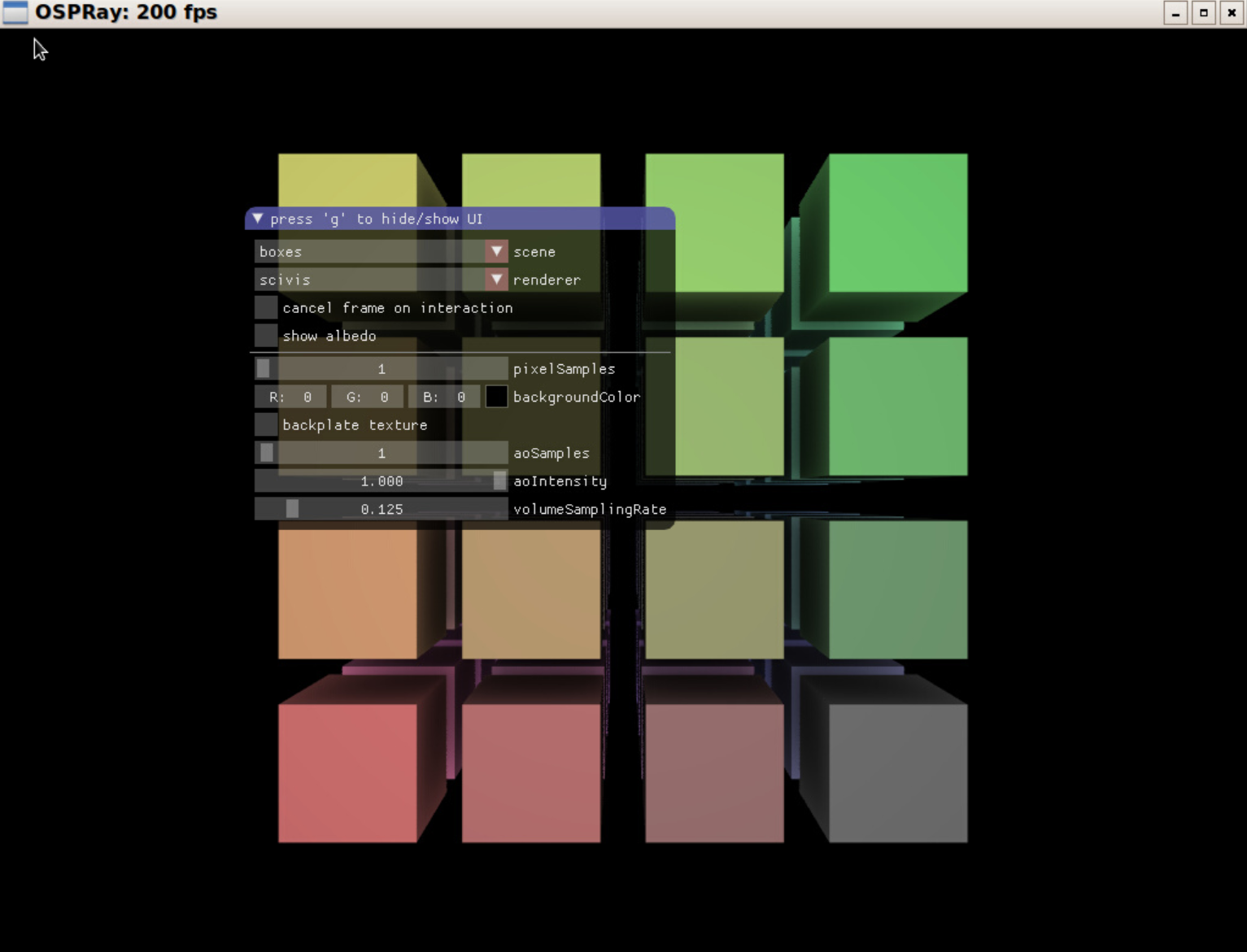
ospExamples application with default boxes scene.

Scenes

Different scenes can be selected from the scenes dropdown and each scene corresponds to an instance of a special detail::Builder struct. Example builders are located in apps/common/ospray_testing/builders/. These builders provide a usage guide for the OSPRay scene hierarchy and OSPRay API in the form of cpp wrappers. They instantiate and manage objects for the specific scene like cpp::Geometry, cpp::Volume, cpp::Light etc.

The detail::Builder base struct is mostly responsible for setting up OSPRay world and objects common in all scenes (for example lighting and ground plane), which can be conveniently overridden in the derived builders.

Renderer

This app comes with four renderer options: scivis, pathtracer, ao and debug. The app provides some common rendering controls like pixelSamples and other more specific to the renderer type like aoSamples for the scivis and ao renderer or maxPathLength for the pathtracer.

The sun-sky lighting can be used in a sample scene by enabling the renderSunSky option of the pathtracer renderer. It allows the user to change turbidity and sunDirection.

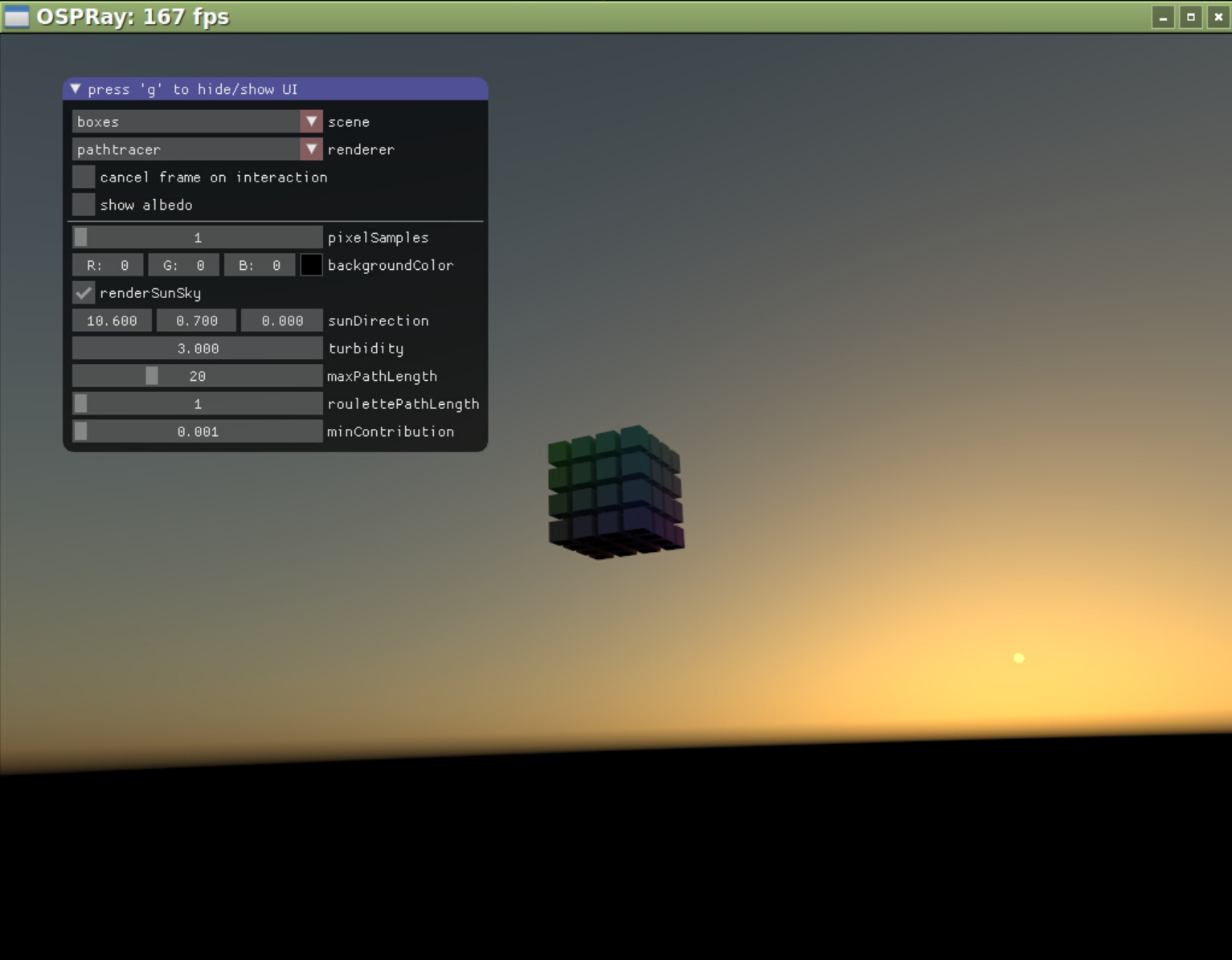
Rendering an evening sky with the renderSunSky option.

ospMPIDistribTutorial

A minimal working example demonstrating how to use OSPRay for rendering distributed data can be found at modules/mpi/tutorials/ospMPIDistribTutorial.c¹⁰.

The compilation process via CMake is the similar to apps/tutorials/ospTutorialFindospray/, with the addition of finding and linking MPI.

To build the tutorial on Linux, build it in a build directory with

mpicc -std=c99 ../modules/mpi/tutorials/ospMPIDistribTutorial.c \
-I ../ospray/include -L . -lospray -Wl,-rpath,. -o ospMPIDistribTutorial

On Windows build it can be build manually in a “build_directory\$Configuration” directory with

cl ..\..\modules\mpi\tutorials\ospMPIDistribTutorial.c -I ..\..\ospray\include -I ..\.. ospray.lib

The MPI module does not need to be linked explicitly, as it is loaded as a module at runtime.

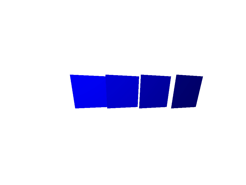
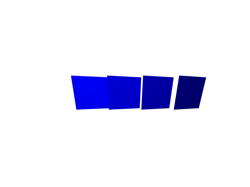
The first frame output by the ospMPIDistribTutorial or C++ tutorial with 4 ranks.

The accumulated frame output by the ospMPIDistribTutorial or C++ tutorial with 4 ranks.

ospMPIDistribTutorialSpheres and ospMPIDistribTutorialVolume

The spheres and volume distributed tutorials are built as part of the MPI tutorials when building OSPRay with the MPI module and tutorials enabled. These tutorials demonstrate using OSPRay to render distributed data sets where each rank owns some subregion of the data, and displaying the output in an interactive window. The domain is distributed in a grid among the processes, each of which will generate a subset of the data corresponding to its subdomain.

In ospMPIDistribTutorialSpheres, each process generates a set of spheres within its assigned domain. The spheres are colored from dark to light blue, where lighter colors correspond to higher ranks.

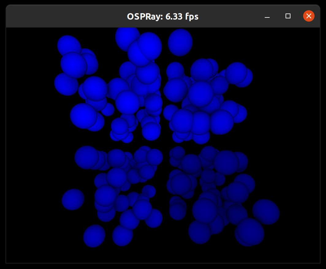
Running ospMPIDistribTutorialSpheres on 4 ranks.

In ospMPIDistribTutorialVolume, each process generates a subbrick of volume data, which is colored by its rank.

Running ospMPIDistribTutorialVolume on 4 ranks.

ospMPIDistribTutorialPartialRepl

The partially replicated MPI tutorial demonstrates how to use OSPRay’s distributed rendering capabilities to render data sets that are partially replicated among the processes. Each pair of ranks generates the same volume brick, allowing them to subdivide the rendering workload between themselves. For example, when run with two ranks, each will generate the same brick and be responsible for rendering half of the image tiles it projects to. When run with four ranks, the pairs of ranks 0,1 and 2,3 will generate the same data and divide the rendering workload for that data among themselves.

The image work subdivision happens automatically, based on which ranks specify the same bounding box for their data, as demonstrated in the tutorial.

The partially replicated distribution is useful to support load-balanced rendering of data sets that are too large to be fully replicated among the processes, but are small enough to be partially replicated among them.

ospMPIDistribTutorialReplicated

The replicated MPI tutorial demonstrates how OSPRay’s distributed rendering capabilities can be used to render data sets that are fully replicated among the ranks with advanced illumination effects. In this case, although the processes are run MPI parallel, each rank specifies the exact same data. OSPRay’s MPI parallel renderer will detect that the data is replicated in this case and use the same image-parallel rendering algorithms employed in the MPI offload rendering configuration to render the data. This image-parallel rendering algorithm supports all rendering configurations that are used in local rendering, e.g., path tracing, to provide high-quality images.

The replicated MPI tutorial supports the same scenes and parameters as the ospExamples app described above.

This mode can be useful when high-quality rendering is desired and it is possible to copy the entire data set on to each rank, or to accelerate loading of a large model by leveraging a parallel file system.

Footnotes

1. This file is usually in ${install_location}/[lib|lib64]/cmake/ospray-${version}/. If CMake does not find it automatically, then specify its location in variable ospray_DIR (either an environment variable or CMake variable). ↩

2. The number of items to be copied is defined by the size of the source array. ↩

3. For consecutive memory addresses the x-index of the corresponding voxel changes the quickest. ↩

4. actually a parallelogram ↩

5. respectively $(127, 127, 255)$ for 8 bit textures and $(32767, 32767, 65535)$ for 16 bit textures ↩

6. including spheres, boxes, infinite planes, closed meshes, closed subdivisions and curves ↩

7. OSPBounds has essentially the same layout as the OSP_BOX3F OSPDataType. ↩

8. If there are multiple ambient lights then their contribution is added. ↩

9. A C++ version that uses the C++ convenience wrappers of OSPRay’s C99 API via include/ospray/ospray_cpp.h is available at apps/tutorials/ospTutorial.cpp. ↩

10. A C++ version that uses the C++ convenience wrappers of OSPRay’s C99 API via include/ospray/ospray_cpp.h is available at modules/mpi/tutorials/ospMPIDistribTutorial.cpp. ↩