class: middle, center, title-slide count: false
.huge.blue[Matthew Feickert]
.huge[(University of Illinois at Urbana-Champaign)]
matthew.feickert@cern.ch
May 20th, 2021
.middle-logo[]
.grid[
.kol-1-4.center[
.circle.width-80[ ]
]
CERN
]
.kol-1-4.center[
.circle.width-80[
Illinois
]
.kol-1-4.center[
.circle.width-80[ ]
]
UCSC SCIPP
]
.kol-1-4.center[
.circle.width-75[
NCSA/Illinois ] ]
.kol-1-2[
- HPC facilities provide an opportunity to efficiently perform the statistical inference of LHC data
- Can pose problems with orchestration and efficient scheduling
- Want to leverage pyhf hardware accelerated backends at HPC sites for real analysis speedup
- Reduce fitting time from hours to minutes
- Deploy a .bold[(fitting) Function as a Service] (FaaS) powered through funcX
- Example use cases:
- Large scale ensemble fits for statistical combinations
- Large dimensional scans of theory parameter space (e.g. pMSSM scans)
- Pseudo-experiment generation ("toys")
]
.kol-1-2[
.center.width-90[
 ]
ATLAS workspace that takes over an hour on ROOT fit in under 1 minute with pyhf on local GPU
]
]
ATLAS workspace that takes over an hour on ROOT fit in under 1 minute with pyhf on local GPU
]

.kol-1-2[
.center.width-50[![]() ]
]
- Pure Python implementation of the
HistFactorystatistical specification for multi-bin histogram-based analysis - Supports multiple computational backends and optimizers (defaults of NumPy and SciPy)
- JAX, TensorFlow, and PyTorch backends can leverage hardware acceleration (GPUs, TPUs) and automatic differentiation
- Possible to outperform C++ implementations of
HistFactory] .kol-1-2[ .center.width-80[ ]
] - High-performance FaaS platform
- Designed to orchestrate scientific workloads across heterogeneous computing resources (clusters, clouds, and supercomputers) and task execution providers (HTCondor, Slurm, Torque, and Kubernetes)
- Leverages Parsl for efficient parallelism and managing concurrent task execution
- Allows users to register and then execute Python functions in "serverless supercomputing" workflow ]
.kol-2-5[
- funcX endpoint: logical entity that represents a compute resource
- Managed by an agent process allowing the funcX service to dispatch user defined functions to resources for execution
- Agent handles:
- Authentication and authorization
- Provisioning of nodes on the compute resource
- Monitoring and management ] .kol-3-5[
.tiny[
from funcx_endpoint.endpoint.utils.config import Config
...

user_opts = {
    "expanse": {
        "worker_init": ". ~/setup_expanse_funcx_test_env.sh",
        "scheduler_options": "#SBATCH --gpus=1",
    }
}

config = Config(
    executors=[
        HighThroughputExecutor(
            label="Expanse_GPU",
            address=address_by_hostname(),
            provider=SlurmProvider(
                "gpu",  # Partition / QOS
                account="nsa106",
                nodes_per_block=1,
                max_blocks=4,
                init_blocks=1,
                mem_per_node=96,
                scheduler_options=user_opts["expanse"]["scheduler_options"],
                worker_init=user_opts["expanse"]["worker_init"],
                launcher=SrunLauncher(),
                walltime="00:10:00",
                cmd_timeout=120,
            ),
        ),
    ],
)
] ]
.kol-1-2[
Example Parsl HighThroughputExecutor config (from Parsl docs) that .bold[funcX extends]
.tiny[
from parsl.config import Config
from libsubmit.providers.local.local import Local
from parsl.executors import HighThroughputExecutor

config = Config(
    executors=[
        HighThroughputExecutor(
            label='local_htex',
            workers_per_node=2,
            provider=Local(
                min_blocks=1,
                init_blocks=1,
                max_blocks=2,
                nodes_per_block=1,
                parallelism=0.5
            )
        )
    ]
)
] .tiny[
- block: Basic unit of resources acquired from a provider
max_blocks: Maximum number of blocks that can be active per executornodes_per_block: Number of nodes requested per blockparallelism: Ratio of task execution capacity to the sum of running tasks and available tasks ] ] .kol-1-2[ .center.width-100[ ]
]- 9 tasks to compute
- Tasks are allocated to the first block until its
task_capacity(here 4 tasks) reached - Task 5: First block full and
5/9 > parallelism
so Parsl provisions a new block for executing the remaining tasks ]
.kol-2-3[ .tiny[
import json
from time import sleep

import pyhf
from funcx.sdk.client import FuncXClient
from pyhf.contrib.utils import download


def prepare_workspace(data, backend):
    import pyhf

    pyhf.set_backend(backend)
    return pyhf.Workspace(data)


def infer_hypotest(workspace, metadata, patches, backend):
    import time
    import pyhf

    pyhf.set_backend(backend)

    tick = time.time()
    model = workspace.model(...)
    data = workspace.data(model)
    test_poi = 1.0
    return {
        "metadata": metadata,
        "CLs_obs": float(
            pyhf.infer.hypotest(test_poi, data, model, test_stat="qtilde")
        ),
        "Fit-Time": time.time() - tick,
    }

...
]
]
.kol-1-3[
- As the analyst user, define the functions that you want the funcX endpoint to execute
- These are run as individual jobs and so require all dependencies of the function to .bold[be defined inside the function]
.tiny[
import numpy  # Not in execution scope

def example_function():
    import pyhf  # Import here

    ...

    pyhf.set_backend("jax")  # To use here
] ]
.kol-2-3[ .tiny[
...

def main(args):

    ...

    # Initialize funcX client
    fxc = FuncXClient()
    fxc.max_requests = 200

    with open("endpoint_id.txt") as endpoint_file:
        pyhf_endpoint = str(endpoint_file.read().rstrip())

    # register functions
    prepare_func = fxc.register_function(prepare_workspace)

    # execute background only workspace
    bkgonly_workspace = json.load(bkgonly_json)
    prepare_task = fxc.run(
        bkgonly_workspace, backend, endpoint_id=pyhf_endpoint, function_id=prepare_func
    )

    workspace = None
    while not workspace:
        try:
            workspace = fxc.get_result(prepare_task)
        except Exception as excep:
            print(f"prepare: {excep}")
            sleep(10)

...
] ] .kol-1-3[
- With the user functions defined, they can then be registered with the funcX client locally
fx.register_function(...)
- The local funcX client can then execute the request to the remote funcX endpoint, handling all communication and authentication required
fx.run(...)
- While the job run on the remote HPC system, can make periodic requests for finished results
fxc.get_result(...)- Returning the output of the user defined functions ]
.kol-2-3[ .tiny[
...

    # register functions
    infer_func = fxc.register_function(infer_hypotest)

    patchset = pyhf.PatchSet(json.load(patchset_json))

    # execute patch fits across workers and retrieve them when done
    n_patches = len(patchset.patches)
    tasks = {}
    for patch_idx in range(n_patches):
        patch = patchset.patches[patch_idx]
        task_id = fxc.run(
            workspace,
            patch.metadata,
            [patch.patch],
            backend,
            endpoint_id=pyhf_endpoint,
            function_id=infer_func,
        )
        tasks[patch.name] = {"id": task_id, "result": None}

    while count_complete(tasks.values()) < n_patches:
        for task in tasks.keys():
            if not tasks[task]["result"]:
                try:
                    result = fxc.get_result(tasks[task]["id"])
                    tasks[task]["result"] = result
                except Exception as excep:
                    print(f"inference: {excep}")
                    sleep(15)

...
] ] .kol-1-3[
- The workflow
fx.register_function(...)fx.run(...)
can now be used to scale out .bold[as many custom functions as the workers can handle]
- This allows for all the signal patches (model hypotheses) in a full analysis to be .bold[run simultaneously across HPC workers]
- Run from anywhere (e.g. laptop)!
- The user analyst has .bold[written only simple pure Python]
- No system specific configuration files needed ]
.kol-1-2[
- .bold[Example]: Fitting all 125 models from
pyhfpallet for published ATLAS SUSY 1Lbb analysis - Wall time .bold[under 2 minutes 30 seconds]
- Downloading of
pyhfpallet from HEPData (local machine) - Registering functions (local machine)
- Sending serialization to funcX endpoint (remote HPC)
- funcX executing all jobs (remote HPC)
- funcX retrieving finished job output (local machine)
- Downloading of
- Deployments of funcX endpoints currently used for testing
- University of Chicago River HPC cluster (CPU)
- NCSA Bluewaters (CPU)
- XSEDE Expanse (GPU JAX) ] .kol-1-2[ .tiny[
feickert@ThinkPad-X1:~$ time python fit_analysis.py -c config/1Lbb.json
prepare: waiting-for-ep
prepare: waiting-for-ep
--------------------
<pyhf.workspace.Workspace object at 0x7fb4cfe614f0>
Task C1N2_Wh_hbb_1000_0 complete, there are 1 results now
Task C1N2_Wh_hbb_1000_100 complete, there are 2 results now
Task C1N2_Wh_hbb_1000_150 complete, there are 3 results now
Task C1N2_Wh_hbb_1000_200 complete, there are 4 results now
Task C1N2_Wh_hbb_1000_250 complete, there are 5 results now
Task C1N2_Wh_hbb_1000_300 complete, there are 6 results now
Task C1N2_Wh_hbb_1000_350 complete, there are 7 results now
Task C1N2_Wh_hbb_1000_400 complete, there are 8 results now
Task C1N2_Wh_hbb_1000_50 complete, there are 9 results now
Task C1N2_Wh_hbb_150_0 complete, there are 10 results now
...
Task C1N2_Wh_hbb_900_150 complete, there are 119 results now
Task C1N2_Wh_hbb_900_200 complete, there are 120 results now
inference: waiting-for-ep
Task C1N2_Wh_hbb_900_300 complete, there are 121 results now
Task C1N2_Wh_hbb_900_350 complete, there are 122 results now
Task C1N2_Wh_hbb_900_400 complete, there are 123 results now
Task C1N2_Wh_hbb_900_50 complete, there are 124 results now
Task C1N2_Wh_hbb_900_250 complete, there are 125 results now
--------------------
...

real	2m17.509s
user	0m6.465s
sys	 0m1.561s
] ]
.kol-1-2[
- Remember, the returned output is just the .bold[function's return]
- Our hypothesis test user function from earlier:
.tiny[
def infer_hypotest(workspace, metadata, patches, backend):
    import time
    import pyhf

    pyhf.set_backend(backend)

    tick = time.time()
    model = workspace.model(...)
    data = workspace.data(model)
    test_poi = 1.0
    return {
        "metadata": metadata,
        "CLs_obs": float(
            pyhf.infer.hypotest(
                test_poi, data, model, test_stat="qtilde"
                )
        ),
        "Fit-Time": time.time() - tick,
    }
] ] .kol-1-2[
- Allowing for easy and rapid serialization and manipulation of results
- Time from submitting jobs to plot can be minutes
.tiny[
feickert@ThinkPad-X1:~$ python fit_analysis.py -c config/1Lbb.json > run.log
# Some light file manipulation later to extract results.json from run.log
feickert@ThinkPad-X1:~$ jq .C1N2_Wh_hbb_1000_0 results.json
{
  "metadata": {
    "name": "C1N2_Wh_hbb_1000_0",
    "values": [
      1000,
      0
    ]
  },
  "CLs_obs": 0.5856783708143126,
  "Fit-Time": 28.786057233810425
}
feickert@ThinkPad-X1:~$ jq .C1N2_Wh_hbb_1000_0.CLs_obs results.json
0.5856783708143126
] ]
.kol-1-2[
- Fit times for analyses using
pyhf's NumPy backend and SciPy optimizer orchestrated with funcX on River HPC cluster (CPU) over 10 trials compared to a single RIVER node - Reported wall fit time is the mean wall fit time of the trials
- Uncertainty on the mean wall time corresponds to the standard deviation of the wall fit times
- Given the variability in resources available on real clusters, funcX config options governing resources requested (.bold[nodes per block] and .bold[max blocks]) offer most useful worker comparison metrics
]
.kol-1-2[
.center.width-100[
 ]
]
]
]

.large[
| Analysis | Patches | Nodes per block | Max blocks | Wall time (sec) | Single node (sec) | ||||
|---|---|---|---|---|---|---|---|---|---|
| Eur. Phys. J. C 80 (2020) 691 | 125 | 1 | 4 | 3842 | |||||
| JHEP 06 (2020) 46 | 76 | 1 | 4 | 114 | |||||
| Phys. Rev. D 101 (2020) 032009 | 57 | 1 | 4 | 612 |
]
.kol-2-5[
- The nature of FaaS that makes it highly scalable also leads to a problem for taking advantage of just-in-time (JIT) compiled functions
- To leverage JITed functions there needs to be .bold[memory that is preserved across invocations] of that function
- Nature of FaaS: Each function call is self contained and .bold[doesn't know about global state]
- funcX endpoint listens on a queue and invokes functions ] .kol-3-5[ .tiny[
In [1]: import jax.numpy as jnp
   ...: from jax import jit, random

In [2]: def selu(x, alpha=1.67, lmbda=1.05):
   ...:     return lmbda * jnp.where(x > 0, x, alpha * jnp.exp(x) - alpha)
   ...:

In [3]: key = random.PRNGKey(0)
   ...: x = random.normal(key, (1000000,))

In [4]: %timeit selu(x)
850 µs ± 35.4 µs per loop (mean ± std. dev. of 7 runs, 1000 loops each)

In [5]: selu_jit = jit(selu)

In [6]: %timeit selu_jit(x)
17.2 µs ± 105 ns per loop (mean ± std. dev. of 7 runs, 100000 loops each)
] .center[50X speedup from JIT] ] .kol-1-1[
- Thoughts for future: Is it possible to create setup and tear down functionality to improve parallelized fitting?
- Setup: Send function(s) to JIT and keep them in state
- Tear down: Once jobs are finished clean up state ]
- Through the combined use of the pure-Python libraries .bold[funcX and
pyhf], demonstrated the ability to .bold[parallelize and accelerate] statistical inference of physics analyses on HPC systems through a .bold[FaaS solution] - Without having to write any bespoke batch jobs, inference can be registered and executed by analysts with a client Python API that still achieves the large performance gains compared to single node execution that is a typical motivation of use of batch systems.
- Allows for transparently switching workflows from .bold[CPU to GPU] environments
- Further performance testing ongoing
- Not currently able to leverage benefits of JITed operations
- Motivates investigation of the scaling performance for large scale ensemble fits in the case of statistical combinations of analyses and large dimensional scans of theory parameter space (e.g. phenomenological minimal supersymmetric standard model (pMSSM) scans)
- All code used public and open source!
class: end-slide, center
.large[Backup]
- "Thing X outperforms ROOT" isn't specific enough to be very helpful - All claims about performance against ROOT: - Made on ROOT `v6.22.02` or earlier - Made given HistFactory models (not against `WSMaker` or something similar) - Still need to be tested against the recent ROOT `v6.24.00` release - For a fitting service like what is being done with funcX fair comparisons are extremely difficult to create, and so aren't reported directly here
-
funcX provides a managed service secured by Globus Auth
-
Endpoints can be set up by a site administrator and shared with authorized users through Globus Auth Groups
-
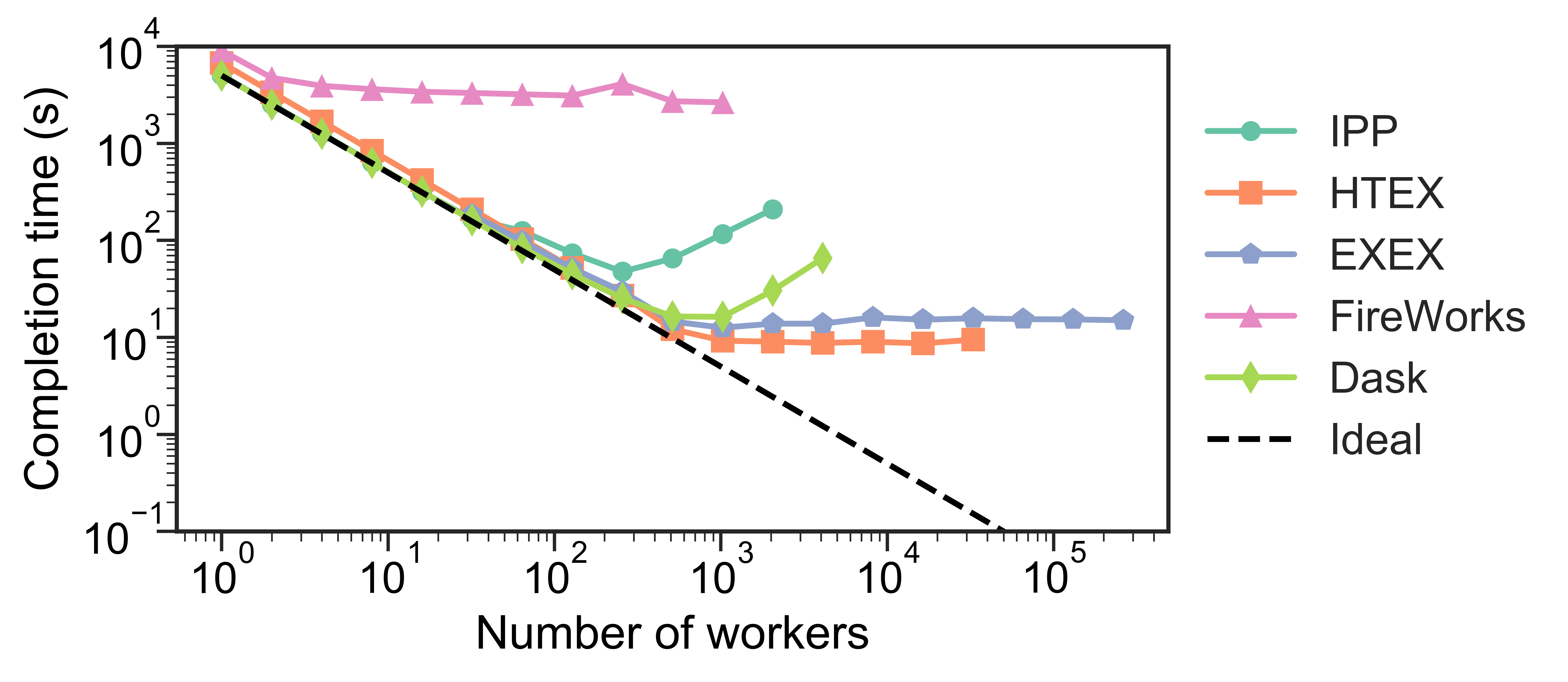
Testing has shown that Dask struggles to .bold[scale up to thousands of nodes], whereas the funcX High Throughput Executor (HTEX) provided through Parsl scales efficiently
 ]
].center.width-100[ ]
]
- Lukas Heinrich, .italic[Distributed Gradients for Differentiable Analysis], Future Analysis Systems and Facilities Workshop, 2020.
- Babuji, Y., Woodard, A., Li, Z., Katz, D. S., Clifford, B., Kumar, R., Lacinski, L., Chard, R., Wozniak, J., Foster, I., Wilde, M., and Chard, K., Parsl: Pervasive Parallel Programming in Python. 28th ACM International Symposium on High-Performance Parallel and Distributed Computing (HPDC). 2019. https://doi.org/10.1145/3307681.3325400
class: end-slide, center count: false
The end.