class: middle, center, title-slide count: false

Distributed statistical inference

with `pyhf` powered by `funcX`

.huge.blue[Matthew Feickert]

.width-02[] matthew.feickert@cern.ch
.width-02[] @HEPfeickert
.width-02[] matthewfeickert

Physics and Astronomy Mini-symposia
[SciPy 2021](https://www.scipy2021.scipy.org/)
July 15th, 2021

Project team

.grid[ .kol-1-4.center[ .circle.width-80[]

Lukas Heinrich

CERN ] .kol-1-4.center[ .circle.width-80[]

Matthew Feickert

University of Illinois
Urbana-Champaign ] .kol-1-4.center[ .circle.width-80[]

Giordon Stark

UCSC SCIPP ] .kol-1-4.center[ .circle.width-75[]

Ben Galewsky

National Center for
Supercomputing Applications/Illinois ] ]

.kol-3-4.center.bold[pyhf Core Developers] .kol-1-4.center.bold.gray[funcX Developer]

We're high energy particle physicists

.kol-1-2.center[
.width-95[] LHC ] .kol-1-2.center[ .width-95[] ATLAS ] .kol-1-1[ .kol-1-2.center[ .width-45[] ] .kol-1-2.center[ .kol-1-2.center[ .width-100[] ] .kol-1-2.center[ .width-85[] ] ] ]

Goals of physics analysis at the LHC

.kol-1-1[ .kol-1-3.center[ .width-100[] Search for new physics ] .kol-1-3.center[
.width-100[]

Make precision measurements ] .kol-1-3.center[ .width-110[[![SUSY-2018-31_limit](figures/SUSY-2018-31_limit.png)](https://atlas.web.cern.ch/Atlas/GROUPS/PHYSICS/PAPERS/SUSY-2018-31/)]

Provide constraints on models through setting best limits ] ]

All require .bold[building statistical models] and .bold[fitting models] to data to perform statistical inference
Model complexity can be huge for complicated searches
Problem: Time to fit can be .bold[many hours]
.blue[pyhf Goal:] Empower analysts with fast fits and expressive models

pyhf: pure-Python HistFactory statistical models

.kol-3-4[

Pure Python implementation of ubiquitous high energy physics (HEP) statistical model specification for multi-bin histogram-based analysis
Supports .bold[multiple computational backends] and optimizers (defaults of NumPy and SciPy)
JAX, TensorFlow, and PyTorch backends can leverage hardware acceleration (GPUs, TPUs) and automatic differentiation
Possible to outperform traditional C++ implementations that are default in HEP
Ways to learn more:

.kol-1-3.center[ .width-100[] ] .kol-1-3.center[ .width-100[] ] .kol-1-3.center[ .width-100[] ] ] .kol-1-4.center[ .width-85[] .width-85[] .width-85[]

.width-50[![JAX](figures/logos/JAX_logo.png)] ]

Functions as a Service natural habitat: Cloud

.kol-1-3[

Cloud service providers give an excellent Functions as a Service (FaaS) platform that can scale elastically
Example: Running pyhf across 25 worker nodes on Google Cloud Platform
- Results being plotted as they are streamed back
- Fit of all signal model hypotheses in analysis takes .bold[3 minutes]!
Powerful resource, but in (academic) sciences experience is still growing
"Pay for priority" model
- fast and reliable
- requires funding even with nice support from cloud providers ] .kol-2-3[

.center.width-70[] .center.small[(GIF sped up by 8x)] ]

(Fitting) FaaS with `pyhf` on HPCs

.kol-1-2[

HPC facilities are more .bold[commonly available] for use in HEP and provide an opportunity to .bold[efficiently perform statistical inference] of LHC data
Can pose problems with orchestration and efficient scheduling
Want to leverage pyhf hardware accelerated backends at HPC sites for real analysis speedup
- Reduce fitting time from hours to minutes
Idea: Deploy a pyhf based .bold[(fitting) Function as a Service] to HPC centers
Example use cases:
- Large scale ensemble fits for statistical combinations
- Large dimensional scans of theory parameter space (e.g. Phenomenological Minimal Supersymmetric Standard Model scans)
- Pseudo-experiment generation ("toys") ] .kol-1-2[ .center.width-90[] Model that takes over an hour with traditional C++ framework fit in under 1 minute with pyhf on local GPU ]

funcX: high-performance FaaS platform

.center.width-30[]

.kol-1-2[

Designed to orchestrate .bold[scientific workloads] across .bold[heterogeneous computing resources] (clusters, clouds, and supercomputers) and task execution providers (HTCondor, Slurm, Torque, and Kubernetes)
Leverages Parsl parallel scripting library for efficient parallelism and managing concurrent task execution
Allows users to .bold[register] and then .bold[execute] Python functions in "serverless supercomputing" workflow ] .kol-1-2[
funcX SDK provides a Python API to funcX service
Controlling "endpoint" and submission machine can be .bold[totally seperate] (communications routed through Globus)
- Allows for "fire and forget" remote execution where you can run on your laptop, close it, and then retrieve output later
Tool in a growing ecosystem of distributed computing
- Currently looking into other tools like Dask.distributed and Dask-Jobqueue as well ]

funcX endpoints deployment

Deployment of funcX endpoints is straightforward
Example: Deployment to University of Chicago's RIVER cluster with Kubernetes

.center.width-100[![carbon_endpoint_startup](figures/carbon_endpoint_startup.png)]

funcX endpoints on HPC

.kol-2-5[

funcX endpoint: logical entity that represents a compute resource
Managed by an agent process allowing the funcX service to dispatch .bold[user defined functions] to resources for execution
Agent handles:
- Authentication (Globus) and authorization
- Provisioning of nodes on the compute resource
- Monitoring and management
Through funcX endpoint config can use expert knowledge of resource to optimize for task ] .kol-3-5[

.tiny[

from funcx_endpoint.endpoint.utils.config import Config
from funcx_endpoint.executors import HighThroughputExecutor
from funcx_endpoint.providers.kubernetes.kube import KubernetesProvider
from funcx_endpoint.strategies import KubeSimpleStrategy
from parsl.addresses import address_by_route

config = Config(
    executors=[
        HighThroughputExecutor(
            max_workers_per_node=1,
            address=address_by_route(),
            strategy=KubeSimpleStrategy(max_idletime=3600),
            container_type="docker",
            scheduler_mode="hard",
            provider=KubernetesProvider(
                init_blocks=0,
                min_blocks=1,
                max_blocks=100,
                init_cpu=2,
                max_cpu=3,
                init_mem="2000Mi",
                max_mem="4600Mi",
                image="bengal1/pyhf-funcx:3.8.0.3.0-1",
                worker_init="pip freeze",
                namespace="servicex",
                incluster_config=True,
            ),
        )
    ],
    # ...
)

] ]

Execution with funcX: Define user functions

.kol-2-3[ .tiny[

import json
from time import sleep

import pyhf
from funcx.sdk.client import FuncXClient
from pyhf.contrib.utils import download


def prepare_workspace(data, backend):
    import pyhf

    pyhf.set_backend(backend)
    return pyhf.Workspace(data)


def infer_hypotest(workspace, metadata, patches, backend):
    import time
    import pyhf

    pyhf.set_backend(backend)

    tick = time.time()
    model = workspace.model(...)
    data = workspace.data(model)
    test_poi = 1.0
    return {
        "metadata": metadata,
        "cls_obs": float(
            pyhf.infer.hypotest(test_poi, data, model, test_stat="qtilde")
        ),
        "fit-time": time.time() - tick,
    }

...

] ] .kol-1-3[

As the analyst user, define the functions that you want the funcX endpoint to execute
These are run as individual jobs and so require all dependencies of the function to .bold[be defined inside the function]

.tiny[

import numpy  # Not in execution scope

def example_function():
    import pyhf  # Import here

    ...

    pyhf.set_backend("jax")  # To use here

] ]

Execution with funcX: Register and run functions

.kol-2-3[ .tiny[

...

def main(args):

    ...

    # Initialize funcX client
    fxc = FuncXClient()
    fxc.max_requests = 200

    with open("endpoint_id.txt") as endpoint_file:
        pyhf_endpoint = str(endpoint_file.read().rstrip())

    # register functions
    prepare_func = fxc.register_function(prepare_workspace)

    # execute background only workspace
    bkgonly_workspace = json.load(bkgonly_json)
    prepare_task = fxc.run(
        bkgonly_workspace, backend, endpoint_id=pyhf_endpoint, function_id=prepare_func
    )

    # retrieve function execution output
    workspace = None
    while not workspace:
        try:
            workspace = fxc.get_result(prepare_task)
        except Exception as excep:
            print(f"prepare: {excep}")
            sleep(10)

...

] ] .kol-1-3[

With the user functions defined, they can then be registered with the funcX client locally
- fx.register_function(...)
The local funcX client can then execute the request to the remote funcX endpoint, handling all communication and authentication required
- fx.run(...)
While the jobs run on the remote HPC system, can make periodic requests for finished results
- fxc.get_result(...)
- Returning the output of the user defined functions ]

Execution with funcX: Scaling out jobs

.kol-2-3[ .tiny[

...

    # register functions
    infer_func = fxc.register_function(infer_hypotest)

    patchset = pyhf.PatchSet(json.load(patchset_json))

    # execute patch fits across workers and retrieve them when done
    n_patches = len(patchset.patches)
    tasks = {}
    for patch_idx in range(n_patches):
        patch = patchset.patches[patch_idx]
        task_id = fxc.run(
            workspace,
            patch.metadata,
            [patch.patch],
            backend,
            endpoint_id=pyhf_endpoint,
            function_id=infer_func,
        )
        tasks[patch.name] = {"id": task_id, "result": None}

    while count_complete(tasks.values()) < n_patches:
        for task in tasks.keys():
            if not tasks[task]["result"]:
                try:
                    result = fxc.get_result(tasks[task]["id"])
                    tasks[task]["result"] = result
                except Exception as excep:
                    print(f"inference: {excep}")
                    sleep(15)

...

] ] .kol-1-3[

The workflow
- fx.register_function(...)
- fx.run(...)

can now be used to scale out .bold[as many custom functions as the workers can handle]

This allows for all the signal patches (model hypotheses) in a full analysis to be .bold[run simultaneously across HPC workers]
- Run from anywhere (e.g. laptop)!
The user analyst has .bold[written only simple pure Python]
- No system specific configuration files needed ]

Scaling of statistical inference

.kol-1-2[

.bold[Example]: Fitting all 125 models from pyhf pallet for published ATLAS SUSY 1Lbb analysis
- DOI: https://doi.org/10.17182/hepdata.90607
Wall time .bold[under 2 minutes 30 seconds]
- Downloading of pyhf pallet from HEPData (submit machine)
- Registering functions (submit machine)
- Sending serialization to funcX endpoint (remote HPC)
- funcX executing all jobs (remote HPC)
- funcX retrieving finished job output (submit machine)
Deployments of funcX endpoints currently used for testing
- University of Chicago River HPC cluster (CPU)
- NCSA Bluewaters (CPU)
- XSEDE Expanse (GPU JAX) ] .kol-1-2[ .tiny[

feickert@ThinkPad-X1:~$ time python fit_analysis.py -c config/1Lbb.json
prepare: waiting-for-ep
prepare: waiting-for-ep
--------------------
<pyhf.workspace.Workspace object at 0x7fb4cfe614f0>
Task C1N2_Wh_hbb_1000_0 complete, there are 1 results now
Task C1N2_Wh_hbb_1000_100 complete, there are 2 results now
Task C1N2_Wh_hbb_1000_150 complete, there are 3 results now
Task C1N2_Wh_hbb_1000_200 complete, there are 4 results now
Task C1N2_Wh_hbb_1000_250 complete, there are 5 results now
Task C1N2_Wh_hbb_1000_300 complete, there are 6 results now
Task C1N2_Wh_hbb_1000_350 complete, there are 7 results now
Task C1N2_Wh_hbb_1000_400 complete, there are 8 results now
Task C1N2_Wh_hbb_1000_50 complete, there are 9 results now
Task C1N2_Wh_hbb_150_0 complete, there are 10 results now
...
Task C1N2_Wh_hbb_900_150 complete, there are 119 results now
Task C1N2_Wh_hbb_900_200 complete, there are 120 results now
inference: waiting-for-ep
Task C1N2_Wh_hbb_900_300 complete, there are 121 results now
Task C1N2_Wh_hbb_900_350 complete, there are 122 results now
Task C1N2_Wh_hbb_900_400 complete, there are 123 results now
Task C1N2_Wh_hbb_900_50 complete, there are 124 results now
Task C1N2_Wh_hbb_900_250 complete, there are 125 results now
--------------------
...

real	2m17.509s
user	0m6.465s
sys	 0m1.561s

] ]

Scaling of statistical inference

.kol-1-2[

.bold[Example]: Fitting all 125 models from pyhf pallet for published ATLAS SUSY 1Lbb analysis
- DOI: https://doi.org/10.17182/hepdata.90607
Wall time .bold[under 2 minutes 30 seconds]
- Downloading of pyhf pallet from HEPData (submit machine)
- Registering functions (submit machine)
- Sending serialization to funcX endpoint (remote HPC)
- funcX executing all jobs (remote HPC)
- funcX retrieving finished job output (submit machine)
Deployments of funcX endpoints currently used for testing
- University of Chicago River HPC cluster (CPU)
- NCSA Bluewaters (CPU)
- XSEDE Expanse (GPU JAX) ] .kol-1-2.center[

.center.width-115[] .center.bold[Click me to watch an asciinema!] ]

Scaling of statistical inference: Results

.kol-1-2[

Remember, the returned output is just the .bold[function's return]
Our hypothesis test user function from earlier:

.tiny[

def infer_hypotest(workspace, metadata, patches, backend):
    import time
    import pyhf

    pyhf.set_backend(backend)

    tick = time.time()
    model = workspace.model(...)
    data = workspace.data(model)
    test_poi = 1.0
    return {
        "metadata": metadata,
        "cls_obs": float(
            pyhf.infer.hypotest(
                test_poi, data, model, test_stat="qtilde"
                )
        ),
        "fit-time": time.time() - tick,
    }

] ] .kol-1-2[

Allowing for easy and rapid serialization and manipulation of results
Time from submitting jobs to plot can be minutes

.tiny[

feickert@ThinkPad-X1:~$ python fit_analysis.py -c config/1Lbb.json
# Returned results saved in results.json
feickert@ThinkPad-X1:~$ jq .C1N2_Wh_hbb_1000_0.result results.json

{
  "metadata": {
    "name": "C1N2_Wh_hbb_1000_0",
    "values": [
      1000,
      0
    ]
  },
  "cls_obs": 0.5856783708143126,
  "fit-time": 24.032342672348022
}

feickert@ThinkPad-X1:~$ jq .C1N2_Wh_hbb_1000_0.result.cls_obs results.json
0.5856783708143126

] ]

FasS constraints and trade-offs

.kol-2-5[

The nature of FaaS that makes it highly scalable also leads to a problem for taking advantage of just-in-time (JIT) compiled functions
- JIT is super helpful for performing pseudo-experiment generation
To leverage JITed functions there needs to be .bold[memory that is preserved across invocations] of that function
FaaS: Each function call is self contained and .bold[doesn't know about global state]
- funcX endpoint listens on a queue and invokes functions
Still need to know and tune funcX config to specifics of endpoint resource
- No magic bullet when using HPC center batch systems ] .kol-3-5[

.tiny[ ```ipython In [1]: import jax.numpy as jnp ...: from jax import jit, random

In [2]: def selu(x, alpha=1.67, lmbda=1.05): ...: return lmbda * jnp.where(x > 0, x, alpha * jnp.exp(x) - alpha) ...:

In [3]: key = random.PRNGKey(0) ...: x = random.normal(key, (1000000,))

In [4]: %timeit selu(x) 850 µs ± 35.4 µs per loop (mean ± std. dev. of 7 runs, 1000 loops each)

In [5]: selu_jit = jit(selu)

In [6]: %timeit selu_jit(x) 17.2 µs ± 105 ns per loop (mean ± std. dev. of 7 runs, 100000 loops each)

]
.center[50X speedup from JIT]
]

---
# Summary

- Through the combined use of the pure-Python libraries .bold[funcX and `pyhf`], demonstrated the ability to .bold[parallelize and accelerate] statistical inference of physics analyses on HPC systems through a .bold[(fitting) FaaS solution]
- Without having to write any bespoke batch jobs, inference can be registered and executed by analysts with a client Python API that still .bold[achieves the large performance gains] compared to single node execution that is a typical motivation of use of batch systems.
- Allows for transparently switching workflows between .bold[provider systems] and from .bold[CPU to GPU] environments
- Not currently able to leverage benefits of .bold[JITed operations]
   - Looking for ways to bridge this
- All [code](https://github.com/matthewfeickert/talk-scipy-2021) used .bold[public and open source] on GitHub!
.kol-1-1[
.kol-1-3.center[
.width-90[[![pyhf_logo](assets/logos/pyhf-logo.png)](https://github.com/scikit-hep/pyhf)]
]
.kol-1-3.center[]
.kol-1-3.center[
<br>
.width-100[[![funcX-light](figures/funcX-light.png)](https://github.com/funcx-faas/funcX)]
]
]

---
class: middle

.center[
# Thanks for listening!
# Come talk with us!

.large[[www.scikit-hep.org/pyhf](https://scikit-hep.org/pyhf/)]
]
.grid[
.kol-1-3.center[
.width-90[[![scikit-hep_logo](https://scikit-hep.org/assets/images/logo.png)](https://scikit-hep.org/)]
]
.kol-1-3.center[
<br>
<!-- .width-90[[![pyhf_logo](https://iris-hep.org/assets/logos/pyhf-logo.png)](https://github.com/scikit-hep/pyhf)] -->
.width-90[[![pyhf_logo](assets/logos/pyhf-logo.png)](https://github.com/scikit-hep/pyhf)]
]
.kol-1-3.center[
<br>
<br>
.width-100[[![iris-hep_logo](figures/iris-hep-4-no-long-name.png)](https://iris-hep.org/)]
]
]

---
class: end-slide, center

.large[Backup]

---
# funcX endpoints on HPC: Config Example

.kol-1-2[
Example Parsl `HighThroughputExecutor` config (from [Parsl docs](https://parsl.readthedocs.io/en/1.1.0/userguide/execution.html#configuration)) that .bold[funcX extends]

.tiny[
```python
from parsl.config import Config
from libsubmit.providers.local.local import Local
from parsl.executors import HighThroughputExecutor

config = Config(
    executors=[
        HighThroughputExecutor(
            label='local_htex',
            workers_per_node=2,
            provider=Local(
                min_blocks=1,
                init_blocks=1,
                max_blocks=2,
                nodes_per_block=1,
                parallelism=0.5
            )
        )
    ]
)

] .tiny[

block: Basic unit of resources acquired from a provider
max_blocks: Maximum number of blocks that can be active per executor
nodes_per_block: Number of nodes requested per block
parallelism: Ratio of task execution capacity to the sum of running tasks and available tasks ] ] .kol-1-2[ .center.width-100[]
9 tasks to compute
Tasks are allocated to the first block until its task_capacity (here 4 tasks) reached
Task 5: First block full and
5/9 > parallelism
so Parsl provisions a new block for executing the remaining tasks ]

View of fitting FaaS Analysis Facility Blueprint

.center.width-100[]

Why look at funcX when Dask is so established?

funcX provides a managed service secured by Globus Auth
Endpoints can be set up by a site administrator and shared with authorized users through Globus Auth Groups
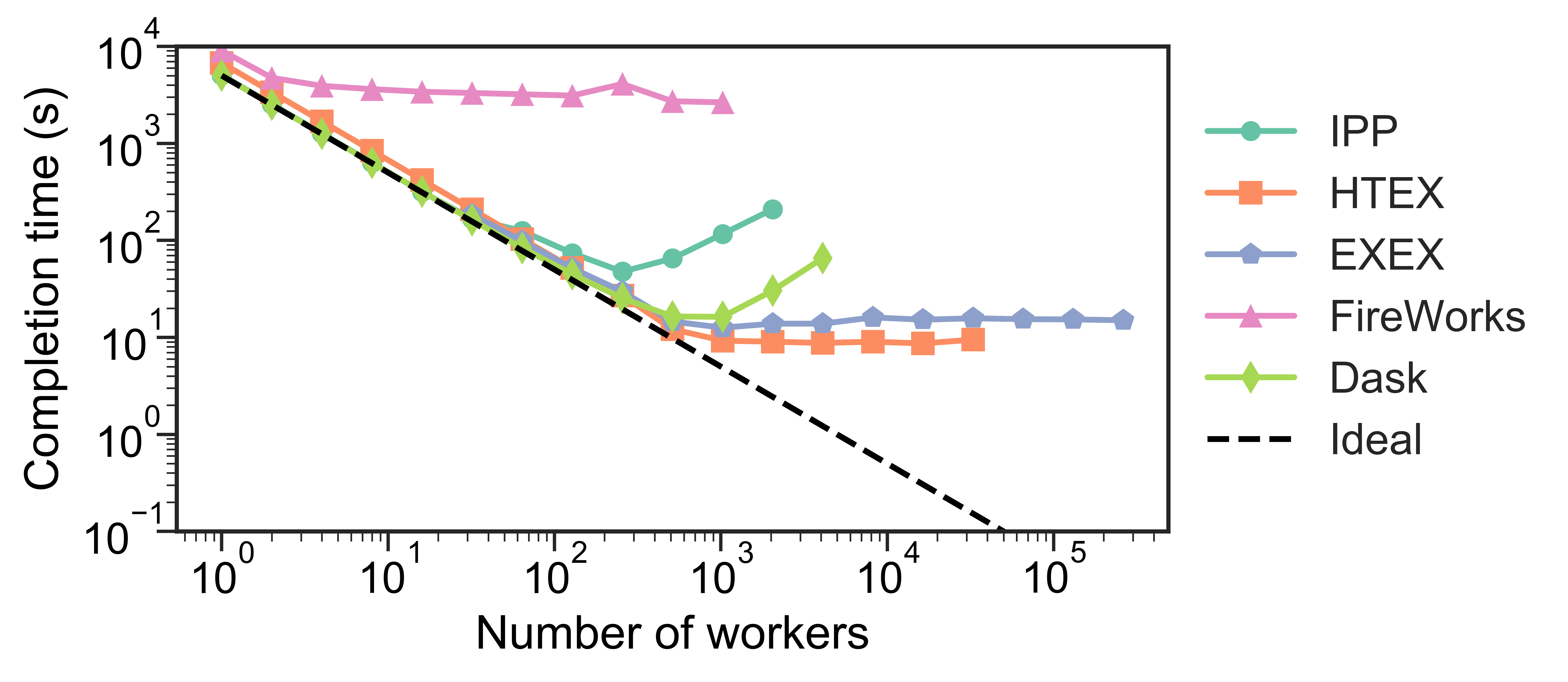
Testing has shown that Dask may not scale well .bold[to thousands of nodes], whereas the funcX High Throughput Executor (HTEX) provided through Parsl scales efficiently

.center.width-80[ Scaling Comparison ]

References

Lukas Heinrich, .italic[Distributed Gradients for Differentiable Analysis], Future Analysis Systems and Facilities Workshop, 2020.
Babuji, Y., Woodard, A., Li, Z., Katz, D. S., Clifford, B., Kumar, R., Lacinski, L., Chard, R., Wozniak, J., Foster, I., Wilde, M., and Chard, K., Parsl: Pervasive Parallel Programming in Python. 28th ACM International Symposium on High-Performance Parallel and Distributed Computing (HPDC). 2019. https://doi.org/10.1145/3307681.3325400

class: end-slide, center count: false

The end.

Provide feedback

Saved searches

Use saved searches to filter your results more quickly

talk.md

talk.md

Distributed statistical inference

with `pyhf` powered by `funcX`

Project team

We're high energy particle physicists

Goals of physics analysis at the LHC

pyhf: pure-Python HistFactory statistical models

Functions as a Service natural habitat: Cloud

(Fitting) FaaS with `pyhf` on HPCs

funcX: high-performance FaaS platform

funcX endpoints deployment

funcX endpoints on HPC

Execution with funcX: Define user functions

Execution with funcX: Register and run functions

Execution with funcX: Scaling out jobs

Scaling of statistical inference

Scaling of statistical inference

Scaling of statistical inference: Results

FasS constraints and trade-offs

View of fitting FaaS Analysis Facility Blueprint

Why look at funcX when Dask is so established?

References

Files

talk.md

Latest commit

History

talk.md

File metadata and controls

Distributed statistical inference

with pyhf powered by funcX

Project team

We're high energy particle physicists

Goals of physics analysis at the LHC

pyhf: pure-Python HistFactory statistical models

Functions as a Service natural habitat: Cloud

(Fitting) FaaS with pyhf on HPCs

funcX: high-performance FaaS platform

funcX endpoints deployment

funcX endpoints on HPC

Execution with funcX: Define user functions

Execution with funcX: Register and run functions

Execution with funcX: Scaling out jobs

Scaling of statistical inference

Scaling of statistical inference

Scaling of statistical inference: Results

FasS constraints and trade-offs

View of fitting FaaS Analysis Facility Blueprint

Why look at funcX when Dask is so established?

References

with `pyhf` powered by `funcX`

(Fitting) FaaS with `pyhf` on HPCs