Xcompact3d Toolbox

QA
Docs
Package
Meta

It is a Python package designed to handle the pre and postprocessing of the high-order Navier-Stokes solver XCompact3d. It aims to help users and code developers to build case-specific solutions with a set of tools and automated processes.

The physical and computational parameters are built on top of traitlets, a framework that lets Python classes have attributes with type checking, dynamically calculated default values, and ‘on change’ callbacks. In addition to ipywidgets for an user friendly interface.

Data structure is provided by xarray (see Why xarray?), that introduces labels in the form of dimensions, coordinates and attributes on top of raw NumPy-like arrays, which allows for a more intuitive, more concise, and less error-prone developer experience. It integrates tightly with dask for parallel computing and hvplot for interactive data visualization.

Finally, Xcompact3d-toolbox is fully integrated with the new Sandbox Flow Configuration. The idea is to easily provide everything that XCompact3d needs from a Jupyter Notebook, like initial conditions, solid geometry, boundary conditions, and the parameters (see examples). It makes life easier for beginners, that can run any new flow configuration without worrying about Fortran and 2decomp. For developers, it works as a rapid prototyping tool, to test concepts and then compare results to validate any future Fortran implementation.

Useful links

• Documentation;
• Changelog;
• Suggestions for new features and bug report;
• See what is coming next (Project page);
• Xcompact3d's repository.

Installation

It is possible to install using pip:

pip install xcompact3d-toolbox

There are other dependency sets for extra functionality:

pip install xcompact3d-toolbox[visu] # interactive visualization with hvplot and others

To install from source, clone de repository:

git clone https://github.com/fschuch/xcompact3d_toolbox.git

And then install it interactively with pip:

cd xcompact3d_toolbox
pip install -e .

You can install additional dependencies as well:

pip install -e .[visu]

Now, any change you make at the source code will be available at your local installation, with no need to reinstall the package every time.

Try it Online

Click on any link above to launch Binder and interact with our notebooks in a live environment!

Examples

• Importing the package:

  import xcompact3d_toolbox as x3d

• Loading the parameters file (both .i3d and .prm are supported, see #7) from the disc:

  prm = x3d.Parameters(loadfile="input.i3d")
  prm = x3d.Parameters(loadfile="incompact3d.prm")

• Specifying how the binary fields from your simulations are named, for instance:

• If the simulated fields are named like ux-000.bin:

  prm.dataset.filename_properties.set(
     separator = "-",
     file_extension = ".bin",
     number_of_digits = 3
  )

• If the simulated fields are named like ux0000:

  prm.dataset.filename_properties.set(
     separator = "",
     file_extension = "",
     number_of_digits = 4
  )

• There are many ways to load the arrays produced by your numerical simulation, so you can choose what best suits your post-processing application. All arrays are wrapped into xarray objects, with many useful methods for indexing, comparisons, reshaping and reorganizing, computations and plotting. See the examples:

• Load one array from the disc:

  ux = prm.dataset.load_array("ux-0000.bin")

• Load the entire time series for a given variable:

  ux = prm.dataset["ux"]

• Load all variables from a given snapshot:

  snapshot = prm.dataset[10]

• Loop through all snapshots, loading them one by one:

  for ds in prm.dataset:
     # compute something
     vort = ds.uy.x3d.first_derivative("x") - ds.ux.x3d.first_derivative("y")
     # write the results to the disc
     prm.dataset.write(data = vort, file_prefix = "w3")

• Or simply load all snapshots at once (if you have enough memory):

  ds = prm.dataset[:]

• It is possible to produce a new xdmf file, so all data can be visualized on any external tool:

• Loop through all snapshots, loading them one by one:

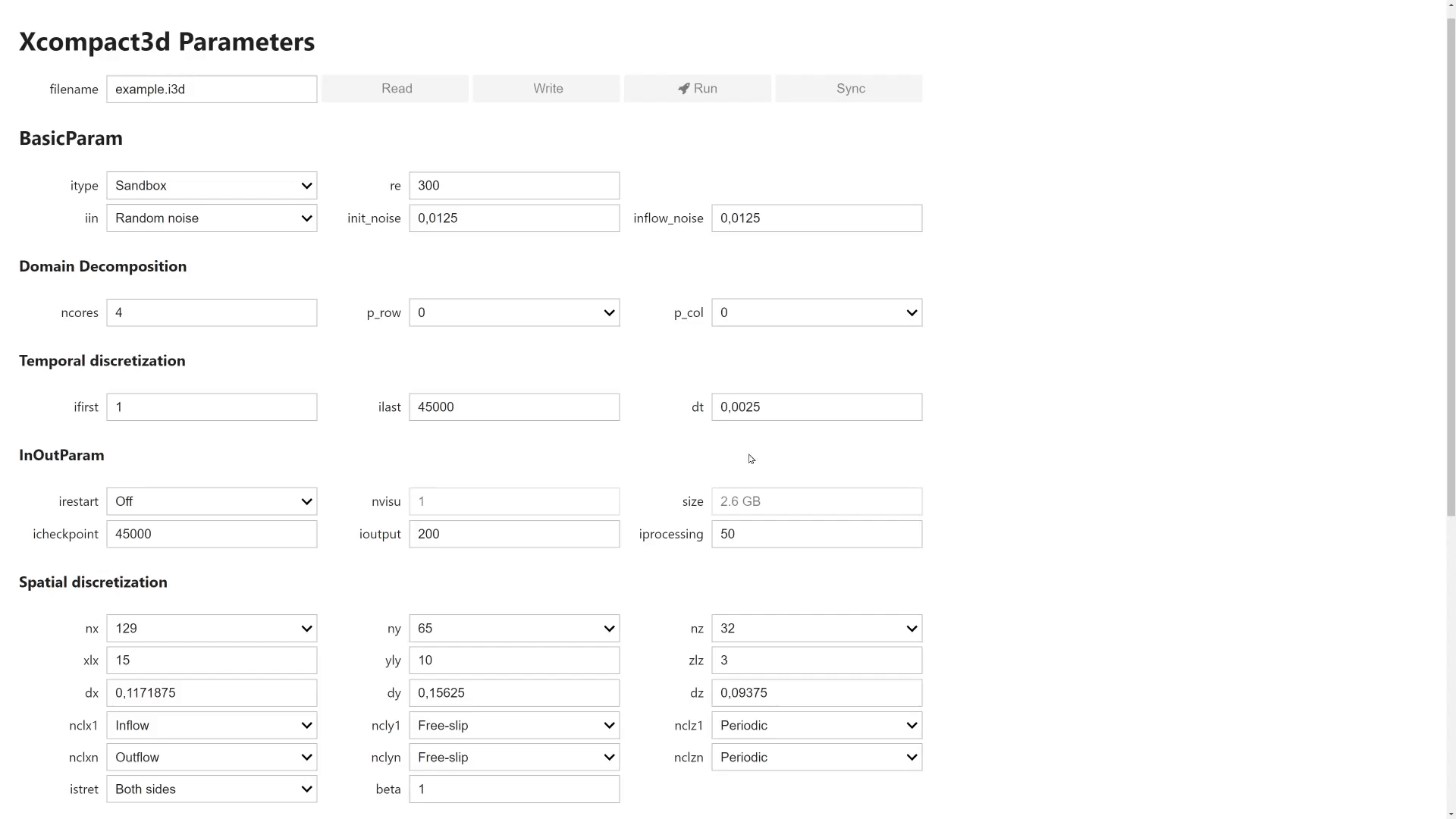
• User interface for the parameters with IPywidgets:

  ds = prm.dataset[:]

• It is possible to produce a new xdmf file, so all data can be visualized on any external tool:

  prm.dataset.write_xdmf()

• User interface for the parameters with IPywidgets:

  prm = x3d.ParametersGui()
  prm

  

Copyright and License

© 2020 Felipe N. Schuch. All content is under GPL-3.0 License.