| How to use | Fundamentals | Example scripts |
![]()
crystalAligner is a computer program for alignment of crystals in a scanning electron microscope. Given one or two crystal orientations (obtained from i.e. EBSD) and associated axes of the microscope coordinate system as alignment objectives, the program optimizes the alignment of the crystal(s) with the microscope coordinate system by global optimization under the constraints of available rotational axes and limits of the microscope stage.
crystalAligner uses MATLAB and the MATLAB-based crystallographic toolbox MTEX under the hood and it therefore utilize crystal symmetries. Furthermore, the determination of the best stage rotation angles is realized with a heuristic optimization algorithm which is robust in finding the global optimum. The crystal alignment can therefore often be optimized to a satisfactory degree even in the case of a standard microscope stage with two rotation axes.
A scientific treatment of the crystallographic aspects and the optimization procedure can be found in the associated research paper. If you like crystalAligner and apply it for your research I would appreciate a citation. Check out the below video for an introduction to crystalAligner.
An introduction to crystalAligner
The program was developed in MATLAB and requires the installation of the crystallographic texture analysis toolbox MTEX as well as the MATLAB global optimization toolboxes. The global optimization toolbox often comes preinstalled with MATLAB or can be obtained separately. If you are not having the toolbox installed, crystalAligner will return an error message related to this. MTEX can be downloaded free of charge and instructions can be found in the video below. crystalAligner has been tested with MTEX versions 4.2.1 to 5.6.0 and MATLAB versions R2014a to R2020a.
To run crystalAligner open MATLAB, navigate to one of the example scripts and execute it. The example script automatically adds the required subdirectories to the MATLAB path. For your own problems it is recommended to make a copy of an example script and adapt it to your setup and optimization problem. Follow some of the examples below to learn how to work with crystalAligner.

If you run a MATLAB version that is older than R2016b you may experience convergence problems in the case of single objective optimization which uses the ga function. The older version of ga is more likely to run into local minima, which can be somewhat mitigated by increasing the initial population size (try increasing the initial population size from 100 to 200 in examples 1 and 4). Multiobjective optimization problems using gamultiobj are not affected by this. Below an example of this is shown, with the ga of the older and newer MATLAB versions left and right, respectively.

It is easiest to follow the examples to learn how to use crystalAligner. However, when working on your own crystal systems, orientations, alignment objectives and microscopes you will need to know how to set up crystalAligner properly. I will therefore go through all parameters that can be defined in the header of the example scripts.
This section specifies the crystal and specimen symmetries, the orientation of your crystal, and of course the crystal directions and microscope axes that should be aligned in the optimization problem. You can define one or two alignment objectives, which are stored in the structure arrays crys(1) and crys(2), respectively. Let's look at the fields that need to be specified:
- SS: This is the specimen symmetry, which can be specified as 'triclinic' or 'orthorhombic' by the MTEX command specimenSymmetry.
- CS: This is the crystal symmetry, which needs a point group as an input. Here we also name the crystal symmetry by specifying the option 'mineral'. This is done with the MTEX command specimenSymmetry. In the case where not all unit axes have the same length, it is also important to state the unit vector lengths when defining the crystal symmetry.
- ori: This is the crystal orientation. It uses the specimen and crystal symmetry as an input. The crystal orientation is usually defined by a set of three Euler angles, which can readily be extracted from EBSD data. There are however plenty of different ways of defining an orientation in MTEX, which you are welcome to use as well.
- alignAx: This is a direction in the specimen coordinate system which is defined as a vector3d instance in MTEX. In the most common cases you will want to align your crystal with the x, y or z directions of your microscope, in which case you can use the global MTEX variables xvector, yvector and zvector.
- Miller: This specifies the crystal direction of crystal plane normal that should be aligned. In MTEX, this is done by using the Miller object. The object simply requires the Miller indicees, the crystal and specimen symmetries, as well as the option 'hkl' or 'uvw' to specify plane normals or directions, respectively. In the case of Miller-Bravais notation using four indecees, the hkil or UVTW are valid options to declare crystal plane normals or directions, respectively. You can define multiple crystal directions by concatenating Miller objects like [Miller1,Miller2,Miller3]. This will sequentially solve multiple optimization problems and is only allowd for the first optimization objective. At last we set the option Miller.opt.useSym to true if we want to use the symmetrically equivalent directions or false if we only want to consider the specific direction.
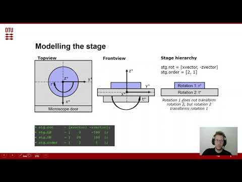
This section specifies the rotation axes and limits of the specimen stage. The settings in the example scripts work for a standard FEI Helios SEM-stage (confirm this for yourself). To demonstrate the concept of the hierarchy of rotation axes, we look at this sample in the image below. We define all rotations with reference to a right-handed cartesian coordinate system x, y, z as shown in the image. In the topview, looking down the optical column of the microscope, we can see that a rotation r is defined around z. The sketched clockwise rotation with positive sign is opposed to the definition of a positive rotation in a right-hand coordinate system. In the front view, looking through the opening chamber door of the microscope, we see that a second rotation, tilt t, is defined around x. This time the rotation is anti-clockwise and therefore has a positive sign in the right-hand coordinate system. The stage hierarchy shows us that r is labeled rotation 1 and t is labeled rotation 2. The numeration is done according to the order of the rotation axes from upper to lowest. The first rotation only rotates the specimen while the second rotation rotates the specimen and the first rotation axis. This hierarchy can be extended to arbitrarily many rotation axes.

The rotation hierarchy is defined in the stg structure in the following way:
- rot: List of the rotation axes in arbitrary order. You can define any kind of 3D-vector here by using vector3d or the global MTEX variables xvector, yvector and zvector. We define whether the rotations around these axes have positive or negative sign with respect to a right-hand coordinate system by the sign in front of the axis. We established that in our above example the tilt around x has a positive sense of rotation while rotation around z has a negative sense of rotation: [xvector; -zvector].
- LB: Lower bound. This defines the lower limits of the rotations, either in terms of the hard limits or personally chosen soft limits. In the above example we don't allow negative tilt and allow full 360° rotation around z by setting the lower bound to -180°: [0, -180]
- UB: Upper bound. This defines the upper limits of the rotations, either in terms of the hard limits or personally chosen soft limits. In the above example we allow tilt up to 20° and full 360° rotation around z by setting the upper bound to 180°: [20, 180]
- order: The order of the rotation axes is defined according to the above explained convention, in our example this is: [2 1]
Here we specify the settings for the genetic algorithm, used to optimize the crystal alignment. This is done in the structure optim:
- order: Order of the optimization problem. This is automatically determined from the parameters of the crystal alignment problem, so do not change this.
- popSz: Size of the population of potential solutions. The larger the population, the more solutions are considered in each generation. A large population should be chosen in the case where the alignment problem is very constrained and therefore determination of a global optimum is complicated. In principle a large population can always be chosen, but it leads to a slow-down of the algorithm which in many cases is unnecessary. Get more information see here.
- funcTol: Optimization option FunctionTolerance, see here.
- maxStallGen: Optimization option MaxStallGenerations, see here.
- iterOut: Writing output for each iteration in subFolder 'iterOut': true/false
- wghtFac: Weighting factors for TOPSIS multiobjective decision making method
- multiCore: Utilization of parallel processing: true/false (not always faster)
- hybridFcn: Use a hybrid function (may speed op convergence but compromise diversity of solution space): true/false
- autoSol: Pick optimum solution automatically by distance of Pareto solution from the optimal solution: true/false
The post-processing parameters include optim.plot which can be set to true or false to activate or deactivate plotting, respectively. They further include the structure FIB to specify parameters of a possible Focussed Ion Beam (FIB) setup. There, parameters will help to calculate the optimized rotation angles at the FIB position and help to estimate trench sizes for TEM lamella preparation at a tilted surface:
- mode: Set this to true or false to get the additional output.
- trench.ang: Default tilt angle for normal alignment of the FIB with the surface
- trench.z: Depth of the trench to be milled in µm
- axs.tilt: Specify which axis in stg.rot is the tilt axis
- axs.rot: Specify which axis in stg.rot is the rotation axis
- Example 1 - Single-objective optimization: Alignment of either of two equivalent crystal plane normals in a cubic crystal
- Example 2 - Multi-objective optimization: Simultaneous alignment of two equivalent crystal directions in a cubic crystal
- Example 3 - Multi-objective optimization: Simultaneous alignment of two equivalent crystal directions of two different crystal structures and orientations
- Example 4 - Single-objective optimization: Refinement of alignment in example 1 by adding a sub-stage
- Example 5 - Multi-objective optimization: Adaption of example 3 to show the use of hexagonal Miller indecees
Single-objective optimization: Alignment of either of two equivalent crystal plane normals in a cubic crystal
Two equivalent crystal plane normals in a cubic crystal with Euler orientation [233 145 33] degrees are aligned in two separate single-objective optimization problems. The crystal could for example represent a ferrite grain in a steel sample. The optimization objective is to align the z-axis of the microscope with either of the {111} or {100} equivalent plane normals. The stage axes setup chosen here represents a standard stage of an FEI scanning electron microscope with chosen soft-limits in the tilt axis of 0 – 20° (the soft limit was chosen to enable further tilting of the aligned crystal for FIB milling). The genetic algorithm is set up to have a population size of 100 individuals. Optional text output for estimating the trench sizes for a FIB lift-out at an inclined surface may be activated. It is found that the {100} can be perfectly aligned while the optimal {111} alignment still deviates about 20° from ideal alignment, caused by the significant constraints by the SEM stage rotation limits (for MATLAB distributions <2016b an optimal solution with non-fulfilled linear constraints might be computed, as explained here.
The expected output is:
Optimization problem 1:
- Rotation around microscope X-axis: 19.9°
- Rotation around microscope Z-axis: -44.6°
- Deviation from ideal alignment in Z-axis: 19.8 °
Optimization problem 2:
- Rotation around microscope X-axis: 15.0°
- Rotation around microscope Z-axis: 133.1°
- Deviation from ideal alignment in Z-axis: 0.0 °
Multi-objective optimization: Simultaneous alignment of two equivalent crystal directions in a cubic crystal
This case is equivalent to application example 1 in the research paper. Here, two equivalent crystal directions in a cubic crystal with Euler orientation [61 42 9] are aligned simultaneously. In this specific application, the crystal represents a β-phase grain in a Ti alloy. The optimization objectives are to align the y-axis of the microscope with any of the <113> equivalent crystal directions and the z-axis of the microscope with any of the <110> equivalent crystal directions. As in example 1, the stage axes represent a standard stage of an FEI scanning electron microscope with chosen soft-limits in the tilt axis of 0 – 20°. The genetic algorithm is set up to have a population size of 100 individuals and no weighting factors applied to the objectives for the choice of the optimal solution. Optional text output for estimating the trench sizes for a FIB lift-out at an inclined surface and plotting of graphs are now activated as well.
The expected output is:
Optimization problem:
- Rotation around microscope X-axis: 6.9°
- Rotation around microscope Z-axis: 132.2°
- Deviation from ideal alignment in Y-axis: 0.1 °
- Deviation from ideal alignment in Z-axis: 0.4 °
FIB lift-out instructions
- Tilt at lift-out position: 6.9°
- Tilt at trenching position: 58.9°
- Alternative: Tilt at trenching position: 45.1° + 180° relative rotation
Trench lengths for 15.0 µm trench depth (z) and 52.0° trench angle:
- Trench length (y) at 'downhill position': 16.6 µm
- Trench length (y) at 'uphill position': 22.7 µm
Multi-objective optimization: Simultaneous alignment of two equivalent crystal directions of two different crystal structures and orientations
This case is equivalent to the application example 2 in the research paper. Here, crystal directions in a cubic and an orthorhombic crystal with Euler orientations [261 43 28] and [175 20 102] are aligned. They represent a β-parent grain and an α’’ martensitic variant in a near-β Ti deformation microstructure. The optimization objectives are to align the x-axis of the microscope with any of the <110> equivalent directions in β and the z-axis of the microscope with the [001] direction of the martensitic α’’. The stage axes represent a standard stage of an FEI scanning electron microscope with chosen soft-limits in the tilt axis of 0 – 20°. The genetic algorithm is set up to have a population size of 500 individuals and no weighting factors applied to the objectives for the choice of the optimal solution.
The expected output is:
Optimization problem:
- Rotation around microscope X-axis: 19.5°
- Rotation around microscope Z-axis: 7.1°
- Deviation from ideal alignment in X-axis: 6.3 °
- Deviation from ideal alignment in Z-axis: 4.1 °
Single-objective optimization: Refinement of alignment in example 1 by adding a sub-stage
In the first example we found that the {100} can be perfectly aligned while the optimal {111} alignment still deviated about 20° from ideal alignment, caused by the significant constraints by the SEM stage rotation limits. Let’s see if we can get an improved allignment for {111} by adding a sub-stage on top of our microscope stage. Compared to the setup for example 1, a rotation axis around the microscope y-axis was added in stg.rot. The rotation limits for this axis are defined as -45 – 45°.
When adding rotation axes it is important to consider the hierarchy of the rotational axes: The sub-stage represents the 1st tilt rotation which should be aligned with the microscope y-axis as an initial position, the microscope z-axis the 2nd rotation and the microscope x-axis the 3rd rotation (stg.order = [3 1 2]). The additional rotational degree of freedom compared to the setup in example 1 leads to perfect alignment of the {111} with the microscope z coordinate axis. Repetitive execution of the code will produce different sets of stage-rotations that lead to the same angular deviation, which is an indicator of multiple ideal solutions for the alignment problem (we are not constrained anymore). As an extension you could try to set the limits of the substage to 45 – 45°, which would simulate the use of a fixed 45° pre-tilt sample holder.
The expected output is:
Optimization problem:
- Rotation around microscope X-axis: 13.4° (not reproducible)
- Rotation around microscope Y-axis: -37.7° (not reproducible)
- Rotation around microscope Z-axis: 28.9° (not reproducible)
- Deviation from ideal alignment in Z-axis: 0.0 °
Multi-objective optimization: Adaption of example 3 to show the use of hexagonal Miller indecees
This example is an adaption of example 3 to demonstrate the use of 4-indicee Miller notation for hexagonal crystals and the distinction of crystal directions and plane normal. Here, a set of crystal plane normals in a cubic crystal and a crystal direction in a hexagonal crystal with Euler orientations [246 36 75] and [91 94 13] are aligned. The optimization objectives are to align the x-axis of the microscope with any of the {011} equivalent plane normals in the cubic crystal and the z-axis of the microscope with the <11-20> equivalent crystal directions of the hexagonal crystal. The stage axes represent a standard stage of an FEI scanning electron microscope with chosen soft-limits in the tilt axis of 0 – 20°. The genetic algorithm is set up to have a population size of 200 individuals and no weighting factors applied to the objectives for the choice of the optimal solution.
The expected output is:
Optimization problem:
- Rotation around microscope X-axis: 8.3°
- Rotation around microscope Z-axis: 147.7°
- Deviation from ideal alignment in X-axis: 10.1 °
- Deviation from ideal alignment in Z-axis: 10.4 °