ArepoVTK: The Arepo Visualization ToolKit

ArepoVTK is a visualization library designed to produce high quality, presentation-ready visualizations of hydrodynamic simulations run with the AREPO code. It can render single images as well as frame sequences for movies from cosmological simulations such as IllustrisTNG as well as idealized test problems and other computational fluid dynamics simulations. It is primarily ray-tracing based, casting through scalar and vector fields defined on an unstructured Voronoi tessellation of space. In this case, piecewise constant/nearest-neighbor (i.e. first order) and linear gradient reconstruction (i.e. second order) are both supported, as is the higher-order natural neighbor interpolation (NNI).

Alternatively, ArepoVTK can disregard the Voronoi mesh and perform N-th nearest neighbor interpolation using an oct-tree structure and various support kernels including the modified Shepard's method (inverse distance weighting), Gaussian, and the usual SPH cubic spline. IDW can also be performed on the natural neighbors of each Voronoi site. As a final alternative, using the dual structure of the Delaunay tessellation, barycentric interpolation on the tetrahedra is available with the Delaunay tessellation field estimator (DTFE) method.

Technically, we implement a high level renderering framework in C++, which is dynamically linked with AREPO to use its existing functionality to e.g. load snapshots, initialize fluid and particle data, and construct the Voronoi mesh and its connectivity structures. Transfer function design is the burden of the user and assumes an expert knowledge of the data present in the snapshots. This is specified, along with all other rendering options, in a configuration file read at run time. Camera support includes: orthographic, perspective, and angular fisheye (180 degree full-dome; 360 degree environmental); camera motion can be animated using keyframes.

ArepoVTK is currently designed to explore novel visualization techniques, i.e. it is highly experimental, easily broken, and assuredly beta software. It is multi-threaded using pthreads, but is not yet multi-node parallelized. It is not interactive.

Future goals include: (i) combining the volume rendering approach with coincident point particle sets, i.e. stars and dark matter, (ii) time interpolation between snapshots, (iii) faster Watson-Sambridge and Liang-Hale algorithms for NNI, (iv) splatting and alternatives to ray-tracing, (v) distributed-memory parallelism with MPI, (vi) GPU acceleration.

Installation

First, make sure you have a recent C++ compiler (gcc or intel). On a standard cluster, load a set of required modules by executing e.g. module load intel gsl fftw hdf5-serial impi. If you are on a laptop or otherwise don't have the module command available, you must install these libraries (consult the AREPO user documentation for more details).

Next, download the ArepoVTK source as well as the public AREPO source:

git clone https://github.com/dnelson86/ArepoVTK.git
cd ArepoVTK/
git clone https://github.com/dnelson86/arepo

Install libpng if it is not already available on your system:

git clone git://git.code.sf.net/p/libpng/code libpng
cd libpng
./configure
make

Build the libarepo.a shared library used within ArepoVTK:

cd ../arepo
make libarepo.a -j

Finally, build ArepoVTK itself:

cd ..
mkdir build
make -j

Executing ./ArepoRT with no options should produce the following output:

      ___           ___           ___           ___           ___                    ___           ___
     /\  \         /\  \         /\  \         /\  \         /\  \                  /\  \         /\  \
    /::\  \       /::\  \       /::\  \       /::\  \       /::\  \                /::\  \        \:\  \
   /:/\:\  \     /:/\:\  \     /:/\:\  \     /:/\:\  \     /:/\:\  \              /:/\:\  \        \:\  \
  /::\~\:\  \   /::\~\:\  \   /::\~\:\  \   /::\~\:\  \   /:/  \:\  \            /::\~\:\  \       /::\  \
 /:/\:\ \:\__\ /:/\:\ \:\__\ /:/\:\ \:\__\ /:/\:\ \:\__\ /:/__/ \:\__\          /:/\:\ \:\__\     /:/\:\__\
 \/__\:\/:/  / \/_|::\/:/  / \:\~\:\ \/__/ \/__\:\/:/  / \:\  \ /:/  /          \/_|::\/:/  /    /:/  \/__/
      \::/  /     |:|::/  /   \:\ \:\__\        \::/  /   \:\  /:/  /              |:|::/  /    /:/  /
      /:/  /      |:|\/__/     \:\ \/__/         \/__/     \:\/:/  /               |:|\/__/     \/__/
     /:/  /       |:|  |        \:\__\                      \::/  /                |:|  |
     \/__/         \|__|         \/__/                       \/__/                  \|__|

   v0.44 (Dec 25 2019). Author: Dylan Nelson (dnelson@uni-heidelberg.de)

Usage: ArepoRT <configfile.txt> [-s snapNum] [-j jobNum] [-e expandedJobNum]

If you see an error message about "error while loading shared libraries", you need to make sure that the paths to the external libraries are specified in the LD_LIBRARY_PATH environment variable, e.g.

export LD_LIBRARY_PATH=$LD_LIBRARY_PATH:$HDF5_HOME/lib:$GSL_HOME/lib:$FFTW_HOME/lib

If you see an error message about "Fatal error in PMPI_Init" or any other strange MPI initialization errors, you may need to unset the following two environment variables (for interactive/shell usage of MPI compiled codes):

unset I_MPI_HYDRA_BOOTSTRAP
unset I_MPI_PMI_LIBRARY

Getting Started

After compilation succeeds, run the first basic test:

./ArepoRT tests/config_2.txt

this should produce a 600x600 pixel image test_frame2.png which is identical to the following:

This is a result of a simple ray-tracing through a small test setup of a uniform grid of 2^3 (i.e. eight) cells within a box [0,1], each with uniform mass. A ninth, central point at [0.5, 0.5, 0.5] is inserted with higher mass. As a result, the gas density field peaks in the center and falls off radially, modulo the imprint of the tessellation geometry. You can get a sense of the geometry with the interactive WebGL Voronoi mesh visualizer.

The transfer function is defined in the configuration file: in this case, there is only one TF added and it is given by the string constant_table Density idl_33_blue-red 0.5 20. The 'constant' means that we will add light to a ray in linear proportion to the 'Density' field it samples. The color of the light is sampled from a 'table', which is specified by its name 'idl_33_blue-red'. This colormap is stretched between a minimum Density value of '0.5' and a maximum of '20' (code units), and outside of this range gas will not contribute to a ray.

---

Next, let's run a permutation of this test on the same "simulation snapshot":

./ArepoRT tests/config_2b.txt

which should produce the image frame2b.png as shown below:

Several configuration choices were changed from the first image. First, the camera was moved such that it views the simulation domain from an oblique angle, rather than directly 'face-on'. The geometry of the bounding box and the single octagonal Voronoi cell in the center of the domain is clear. Second, we have changed the transfer function to constant Density 1.0 0.2 0.0 which is even simpler than above: a fixed color specified by the RGB triplet {R=1, G=0.2, B=0} (i.e. orange) is added to a ray each time it samples gas 'Density', weighted by the value of that density. Finally, we have changed the viStepSize parameter from zero to 0.05. If viStepSize = 0, then ArepoVTK samples each Voronoi cell exactly once, at the midpoint of the line segment defined by the two intersection points of a ray as it enters and exits that cell. On the other hand, if viStepSize > 0 as in the second example, we take strictly step along each ray and take equally spaced samples 0.05 (world space, i.e. code units) apart.

Note that the lines of the bounding box, Delaunay tetrahedra, and Voronoi polyhedra (if drawn) are added in a final pass, rasterization phase. Thus they are not (yet) ray-traced, i.e. cannot be occluded by density along the line of sight.

---

Moving on to a cosmologically interesting use case, we will run and analyze the output of the AREPO example cosmo_box_star_formation_3d. This is a 32^3 gravity + hydrodynamics simulation (i.e. about 32,000 total gas cells) of a small, 7.5 Mpc/h cosmological volume. You can execute this yourself by

cd arepo/examples/
./test.py --print-all-output --no-cleanup cosmo_box_star_formation_3d

this takes about 20-30 minutes to run (on 16 cores). It will produce, among other outputs, the z=0 snapshot: arepo/run/examples/cosmo_box_star_formation_3d/output/snap_005.hdf5. If you don't want to wait that long, you can skip running this test and download the HDF5 snapshot file directly:

mkdir -p arepo/run/examples/cosmo_box_star_formation_3d/output
wget -P !$ https://www.tng-project.org/files/arepo_tests/cosmo_box_star_formation_3d/snap_005.hdf5

Now, we will execute a render to highlight the temperature structure of the evolved intergalactic medium:

./ArepoRT tests/config_cosmo_box.txt

which should produce the image frame_cosmo_box.png as shown below:

here we have switched away from an orthographic projection by setting cameraType = perspective, placing the camera at a distance from the box, pointed towards its center, and with a field of view of 18 degrees. We also use a constant viStepSize = 20 (i.e. code units, ckpc/h in this case), which provides a better sampling of our narrow gaussian transfer functions. You can try setting nTreeNGB = 16 to skip the Voronoi mesh construction and switch to a tree-based interpolation (with the same step size), or try setting viStepSize = 0 to see the impact of only one sample per Voronoi cell, at this rather low resolution.

---

As a final example, consider a cutout of a single galaxy from the high-resolution TNG100-1 cosmological simulation -- you will need a user account, and to be logged in, to download this data. In particular, we will take subhalo 480230 at z=0 which is the central galaxy of a dark matter halo with a mass similar to our own Milky Way. Download a particle cutout of the positions, masses, densities, and magnetic field strength of all the gas cells in the subhalo (this is all we need) with the following link:

https://www.tng-project.org/api/TNG100-1/snapshots/99/subhalos/480285/cutout.hdf5?gas=Coordinates,Masses,MagneticField,Density

Place the resulting cutout_480285.hdf5 file into the ArepoVTK/ directory, and execute a render:

./ArepoRT tests/config_tng100_cutout.txt

which should produce the image frame_tng100_cutout.png as shown below:

here we have switched to a tree-based sampler, sampling every 0.1 kpc, with a transfer function defined by six discrete Gaussian components. Five of these trace density in dark colors, revealing gaseous spiral arms of a disk-like galaxy which is nearly edge-on. The last, in red, shows the location and structure of the magnetic field where it has a value of roughly 0.1 microGauss. To render this cutout from the large 75 cMpc/h cosmological (periodic) volume, we have shifted all the gas cells with recenterBoxCoords = 8361 30797 14480 which repositions the galaxy, as defined by its SubhaloPos, to the center of our visualization box of 2 cMpc/h.

We have also set projColDens = true in this case, which produced an additional output file frame_cosmo_box.png.hdf5. This holds the raw line-of-sight integrals for available fluid quantities. We can inspect this file as

$ h5ls -r frame_tng100_cutout.png.hdf5

/                        Group
/Density                 Dataset {1280, 720}
/Entropy                 Dataset {1280, 720}
/Metal                   Dataset {1280, 720}
/SzY                     Dataset {1280, 720}
/Temp                    Dataset {1280, 720}
/VelMag                  Dataset {1280, 720}
/XRay                    Dataset {1280, 720}

while Density stores integrated column density, the other fields store Density*pathLength weighted quantities. A simple python script like the following will visualize such an output:

import h5py
import numpy as np
import matplotlib.pyplot as plt

with h5py.File('frame_tng100_cutout.png.hdf5','r') as f:
    dens = f['Density'][()]

fig = plt.figure(figsize=[12, 8])
ax = fig.add_subplot(111)

plt.imshow(np.log10(np.flip(dens,axis=1).T), origin='lower', interpolation='nearest', aspect='auto')
plt.colorbar(label='Gas Column Density')
fig.tight_layout()
fig.savefig('frame_tng100_density.png', dpi=75)
plt.close(fig)

which shows the simultaneously derived gas column density map (e.g. in units of Msun/kpc^2).

---

Gallery of Examples

Previous use cases of ArepoVTK, showing some of the breadth of its possible visualization outputs:

• All of the gas images of the Illustris Explorer were generated with ArepoVTK, using the natural neighbor interpolation (NNI) method. The configuration files are available under examples/illustris_box*.

• The Universe in Gas (vimeo) video was made with ArepoVTK, showing gas iso-density and iso-temperature contours within a 20 Mpc/h cosmological volume, each using a set of gaussian_table transfer functions. The configuration files are available under examples/cosmoRot*.

• Stirring Coffee with a Spoon in 3D (vimeo) video was made with ArepoVTK, using gaussian transfer functions on gas density. It is made up of three sequences: the initial rotation, the time-evolving sequence, and the ending. The configuration files are available under examples/spoon*.

• Figure 13 of Nelson et al. (2016) shows gas iso-temperature contours around a single galaxy halo. The configuration files are available under examples/zoom_Nelson16*.

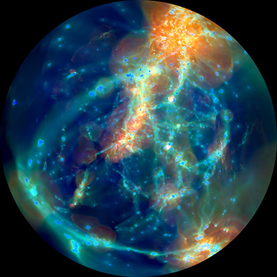
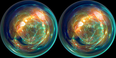
• The 4K and 8K 180 degree fulldome animation of the Illustris temperature evolution were made with ArepoVTK, as was the full 360 degree stereoscopic render (left/right) meant for a HMD like the Oculus Rift. These are picture above. The configuration files are available under examples/illustris_subbox0*.

• A gallery of test images during development is available on the ArepoVTK Development Gallery.

Acknowledgments, Contributing, and Contact

The principal author of ArepoVTK is Dylan Nelson (dnelson@uni-heidelberg.de). If you use this code in a publication, please cite the Nelson et al. (2013) paper where it first made its appearance.

Please contact us with any questions or comments. If you make any changes, updates, fixes, or improvements to this code, please consider making your efforts available to the broader community by contributing back to this project. The most effective way to do so is by submitting an Issue or Pull Request on github.

Reference and Usage

Input and Output

• imageFile - specify the name (and path) of the image to save, should be .tga or .png extension.
• filename - specify the name (and path) of the input AREPO snapshot to load.
• paramFilename - specify the name (and path) of the input AREPO parameterfile.
• writeRGB8bit - true or false, output a 8 bit-depth PNG image (default: true)
• writeRGB16bit - true or false, output a 16 bit-depth PNG image

Transfer Function

• addTF_{N} {spec}

A transfer function is built up from one or more specifications {spec}, each of which is a string:

• constant {field} {colormap}
• constant {field} {R} {G} {B}
• gaussian {field} {mean} {sigma} {colormap}
• gaussian {field} {mean} {sigma} {R} {G} {B}
• tophat {field} {min} {max} {colormap}
• tophat {field} {min} {max} {R} {G} {B}
• constant_table {field} {colormap} {ctMin} {ctMax}
• tophat_table {field} {colormap} {ctMin} {ctMax} {min} {max}
• gaussian_table {field} {colormap} {ctMin} {ctMax} {mean} {sigma}
• linear {field} {min} {max} {colormap_start} {colormap_end}
• linear {field} {min} {max} {R0} {G0} {B0} {R1} {G1} {B1}

Here {field} is the snapshot property to apply to (e.g. Density), and {min} and {max} refer to the value of that quantity (in code units). If specified, {colormap} is the name of a colormap to use and/or sample from. The _table transfer functions sample from a discrete colormap using quantity bounds {ctMin} and {ctMax}.

If using manual specification of {R,G,B} color triplets, these should be in floating point values between 0.0 and 1.0.

• rgbAbsorb - if nonzero enable line-of-sight attenuation/occlusion, {R} {G} {B} triplet. This factor modulates the physical gas density integral along each ray. If the color triplet is the same for all channels, attenuation is monochromatic, otherwise certain colors will be attenuated more than others.

Camera

• imageXPixels - image width (e.g. 800, 1920).
• imageYPixels - image height (e.g. 800, 1080).
• swScale - multiplicative scale factor by which to adjust the size of the view window (i.e. to set the field of view for orthographic renders).
• cameraType - orthographic, perspective, environmental, fisheye
• cameraFOV - field of view (must be zero for orthographic, >0<180 for perspective, 360 for environmental).
• cameraPosition - location of the camera in space, {x} {y} {z} coordinate triplet.
• cameraLookAt - location that the camera looks at in space, {x} {y} {z} coordinate triplet.
• cameraUp - vector denoting the "up" direction of the camera, {x} {y} {z} coordinate triplet.

Animation and Keyframes

• startFrame - for multi-frame renders, start at which frame? (default: 0).
• numFrames - leave at 1 to render a single frame.
• timePerFrame - establish the unit of "time", with respect to the frame number.
• minScale - for multi-frame renders, generally want to fix the range for the mapping into 8bit or 16bit color space, to avoid rapid flickering as the physical minima/maxima change with each frame.
• maxScale - as above, but the maximum (of the color channels).
• minAlpha - as above, but the minimum of the alpha channel.
• maxAlpha - as above, but the maximum of the alpha channel.

Key frames are added with a series of string specifications, similar to transfer functions:

• addKF_{N} {startTime} {stopTime} {quantity} {stopVal} {interpMethod}

where currently {quantity} can be one of cameraX, cameraY, cameraZ, lookAtX, lookAtY, lookAtZ, rotXY, rotXZ and {interpMethod} can be one of linear, quadratic_inout, the latter being a smooth easing function.

Note that a multi-frame sequence could render a time-evolving series of simulation snapshots, or it could render a time-static (i.e. single snapshot) scene. To achieve the former, you can replace the actual snapshot number in {filename} with "NUMM", and then pass in a snapshot number with the -s command-line option. This could, for example, increment simultaneously with the frame number, or else a more complex relationship can be established.

Render Execution, Data Loading, Masking, Multi-Job Renders

• nCores - number of CPU cores to use for multi-threading (1 = serial).
• nTasks - number of independent tasks to decompose the render into, which are then distributed among the threads.
• totNumJobs - if specified and >1, then we are splitting a single render into many independent jobs by subdividing the image plane. For example, if this parameter is 64, then each job will be responsible for 1/64th of the total number of pixels, and each will have an extent of 1/8 of the total along each direction. The spatial domain is decomposed and only a subset of cells are loaded which are sufficient to reconstruct the Voronoi mesh traced by rays from this job alone (see 'mask' below). The current job number is specified by the -j command-line option, e.g. by passing -j ${SLURM_ARRAY_TASKID} in a batch script.
• jobExpansionFac - if {1,2,4}, then exponentiate the totNumJobs parameter by this value. For instance, in the above example of totNumJobs=64 then setting 2 here would result in 4096 total 'expanded' jobs. These subdivide each task further, e.g. for very expensive renderings, while the load decomposition is unchanged and still set by the original totNumJobs. The current expanded job number is specified by the -e command-line option.
• readPartType - particle type to read from snapshot (0 = gas, 1 = dark matter). Currently only one particle type can be loaded and visualized at once.
• maskFileBase - if specified, create and use maskfile for job-based frustum culling (if totNumJobs>1).
• maskPadFac - if using job-based frustum culling, the padding factor (additive, code units) to surround each domain decomposition by. For example, if using an orthographic camera parallel to a box axis, a 75 cMpc/h box with totNumJobs=100 would effectively be decomposed into 7.5 x 7.5 x 75 Mpc/h thin columns/skewers. With maskPadFac = 1000 a 1 cMpc/h ghost buffer would be added to the first two dimensions, which would generally be sufficient to accurately reconstruct the Voronoi mesh.
• recenterBoxCoords - shift the snapshot to center the given {x} {y} {z} position at the middle of the box
• takeLogDens - convert Density from linear to log (code units)
• takeLogUtherm - convert Utherm (or temperature) from linear to log
• convertUthermToKelvin - convert Utherm into Kelvin

Interpolation/Sampling

• viStepSize - if zero, one sample per Voronoi cell. if positive, fixed sample spacing in world space. if negative, should be integer, then adaptive number of sub-samples per cell.
• nTreeNGB - number of nearest neighbors to use for kernel sampling. If zero or omitted, then a Voronoi mesh based sampling is performed. If >0, then no mesh is constructed, and viStepSize must be specified and nonzero.
• rayMaxT - maximum length of rays before termination. If zero (by default), then integrate rays until they exit the simulation box.

Note that, for efficiency reasons, the interpolation algorithm is chosen via preprocessor definition in ArepoRT.h, and the user should choose exactly one of the following:

• NATURAL_NEIGHBOR_INTERP - using the Voronoi mesh, derive a local estimate of the quantity using the Natural Neighbor Interpolation method using "Sibson weights". That is, we take a weighted sum over the parent cell and its natural neighbors, where the weight on each is the fraction of each cell's volume which is stolen if a new Voronoi generating site were to be inserted at the sample point. Note the following properties: the interpolant equals the cell values exactly at their generating sites, the reconstruction is C^2 continuous across cell boundaries, no local minima/maxima are introduced which are not already present, and the weights do not depend only on distance i.e. the interpolant is not spherically symmetric, but rather adapts to irregular point distributions.
• NATURAL_NEIGHBOR_IDW - using the current cell and its natural neighbor as defined by the Voronoi mesh, use the Inverse Distance Weighting scheme with these points and a power parameter of POWER_PARAM.
• NATURAL_NEIGHBOR_SPHKERNEL - using the current cell and its natural neighbor as defined by the Voronoi mesh, use the normal SPH cubic spline kernel with support h defined by HSML_FAC times the distance from the sample point to the furthest natural neighbor.
• NNI_WATSON_SAMBRIDGE - using the Voronoi mesh, NNI is performed with the Watson-Sambridge algorithm.
• NNI_LIANG_HALE - using the Voronoi mesh, NNI is performed with the Liang-Hale algorithm (not implemented).
• DTFE_INTERP - using the Delaunay tessellation, apply the Delaunay tessellation field estimator method.
• CELL_GRADIENTS_DENS - using the Voronoi mesh, linearly reconstruct (i.e. at second order) the value of the quantity at the sample point using the LSF-derived gradients.
• CELL_PIECEWISE_CONSTANT - using the Voronoi mesh, the cell-wide constant value of a quantity is taken. This is nearest neighbor (i.e. first order) interpolation.

Further options:

• NO_GHOST_CONTRIBS - only for SPHKERNEL, do not use ghosts for hsml/TF (i.e. for reflective BCs but we are doing periodic meshing, the ghosts are incorrect and should be skipped)
• NNI_DISABLE_EXACT - for brute-force NNI disable exact geometry computations
• NATURAL_NEIGHBOR_INNER - for IDW, SPHKERNEL or NNI, do "neighbors of neighbors", i.e. extend the search and sampling from immediate neighbors of the parent cell to all neighbors of those neighbors.
• BRUTE_FORCE - for IDW or SPHKERNEL, calculate over all NumGas in the box (instead of N-nearest)
• POWER_PARAM - exponent of distance, greater values assign more influence to values closest to the interpolating point, approaching piecewise constant for large POWER_PARAM.
• HSML_FAC - use <1 for more smoothing, or >1 for less smoothing (at least some neighbors will not contribute, and if this is too big, the containing cell may also not contribute)

Line and Geometry Rendering

• drawBBox - draw bounding box of simulation domain
• drawTetra - draw lines for every Delaunay tetrahedron
• drawVoronoi - draw lines for every Voronoi face
• drawSphere - draw all-sky spherical test grid (for fisheye camera)

Raw Integrals and Non-Image (Scientific) Output

• projColDens - output raw integrals in addition to an image (i.e. no transfer function applied). The result is a HDF5 file {imageFile}.hdf5 with groups for each physical property and corresponding datasets Array which have dimensions {imageXPixels,imageYPixels}. Note that using this option disables early ray termination.

Version Roadmap

Current Version: 0.44.alpha1

+v0.1

• program shell and commandline functionality
• radiative transfer framework:
• pts, vector, matrices, rays, bboxes
• camera: ortho projection, LookAt
• stratified (no jitter or MC) sampler
• volume emission (no scattering) integrator
• renderer, task/image plane subdivision
• image output: raw text floats / TGA
• volumegrid input: "debug" scene descriptor format

+v0.2

• interface with Arepo
• init and snapshot loading
• acquire mesh construction and connectivity - wireframe tetra/bounding box rendering
• wu's line algorithm

+v0.3

• voronoi ray casting
• cell averaged constant
• gradients
• attenuation via optical depth along LOS
• transfer function on a single quantity
• configuration file

+v0.35

• large snapshot support and optimization
• use treefind for entry cells
• handle local ghosts
• 128^3 cosmo rendering
• parallel (threads) on shared memory node

+v0.39

• external colortables
• voronoi cell algorithm
• SPH kernel and IDW of natural neighbors interp methods
• tetra mesh walking
• DTFE
• use internal DC connectivity instead of alternative Sunrise

+v0.4

• multiple frames on single snapshot
• camera path splining/tweening in space, orbits
• fix NNI auxMesh allocation per task instead of per thread

+v0.41

• support for SphKernel and IDW using N-nearest neighbor spheres using NGBTree searches, skip all mesh related tasks including construction and memory overhead

+v0.42

• calculate raw line integrals (do not apply TF) in addition to images
• goal: rendering 1820^3 box
• custom read_ic() with selective loading of only particles in camera frustum
• split camera/image into subchunks, each handled by a separate instance
• maskfile approach to precompute which particles each instance needs to load

+v0.43

• expanded job subdivision
• adaptive spatial stepping with tree based ray tracing

+v0.44

• within custom loading, load DM, Stars, and BHs for rendering (one at a time)
• transfer functions fields for each that make sense for Illustris
• fisheye (180 deg) and environment (360 deg) non-linear cameras
• QuadIntersectionIntegrator (based on single-pass wireframe rendering)
• remove RasterizeLine approach, do bbox lines inside rays based on bbox intersection
• attenuation based on ray optical depth before reaching line

+v0.45

• visualization voronoi mesh based within rays upon each edge intersection
• "splat" integrator via disc intersection testing + kdtree?
• stars: use BC03 stellar photometric tables for U,B,V,K,g,r,i,z band images

+v0.46

• keyframe transfer function settings
• time navigation (multiple snapshots, time interpolation)
• subboxes: render bbox's, update from disk at different interval than fullbox
• movie pipeline
• frame metadata (XML/MKV container?)

+v0.47

• fix/verify exact NNI
• Watson-Sambridge NNI
• Liang-Hale NNI

+v0.48

• load group catalogs, merger trees
• track halos in time

+v0.49

• 2D transfer functions, e.g. f(rho,T)
• derived fields for TFs (e.g. temp, coolingrate)
• johnston convolved planck BB temp emission TF

+v0.50

• remove dependency on libpng with https://lodev.org/lodepng/
• custom memory downsizing (minimize P,SphP)
• robust restart functionality
• load multiple particle types simultaneously: gas/dm, gas/stars
• multiple meshes (e.g. allow DM NNI and gas NNI in TF)

+v0.55

• parallel (MPI) on distributed memory cluster
• handle foreign ghosts
• exchange_rays() type approach

+v0.6

• interactive component (OpenGL)
• alternative/quick rendering modes (splatting)
• navigation
• movie setup
• (single node only)
• GUI on node=0 as client (openWindow=true)

+v0.61

• GPU acceleration (ray tracing)?
• intersection acceleration? (BVH / kdTree)
• memory optimizations (wipe out / rearrange some Arepo stuff)
• speed optimizations?
• discrete NNI on GPU (sub-blocks to meeting sampling requirement)

other

• light sources (star particles)?
• single scattering volume integrator (MC)?
• DOF/motion blur?