Skip to content
New issue

Have a question about this project? Sign up for a free GitHub account to open an issue and contact its maintainers and the community.

By clicking “Sign up for GitHub”, you agree to our terms of service and privacy statement. We’ll occasionally send you account related emails.

Already on GitHub? Sign in to your account

Accuracy of adjoint gradients in 3D #2757

Open
oskooi opened this issue Jan 12, 2024 · 6 comments
Open

Accuracy of adjoint gradients in 3D #2757

oskooi opened this issue Jan 12, 2024 · 6 comments

Comments

@oskooi
Copy link
Collaborator

oskooi commented Jan 12, 2024

edit (1/11): updated script with suggestion to disable subpixel smoothing in MaterialGrid (on by default) from @smartalecH which significantly improves accuracy.

This is an initial attempt to verify the accuracy of the adjoint gradients in 3D. Once we are able to get this example working, we can consider converting it into a unit test for #2661 as well as a tutorial example.

The example involves a power splitter (shown in the schematic below) at $\lambda$ = 1.55 μm for a silicon waveguide on a silicon dioxide substrate. This particular SOI waveguide is identical to an existing tutorial with the schematic and band diagram also shown below. The nice thing about the power splitter is that it is an extension of a similar example in 2D and can be modified to use various types of objective arguments (EigenmodeCoefficient, FourierFields, LDOS) and a broad bandwidth objective function. The design region is a 2D grid with the pixels extruded in the $z$ direction. The example uses either a constant or random design region. The entire simulation runs in about 25 minutes using 3 Xeon 4.2 GHz cores.

The test involves the usual comparison of the directional derivative computed using (1) a brute-force finite difference and (2) the adjoint gradient. (This calculation is similar to the 2D simulation of a 1D grating in #2054 (comment).) The MPB output of the simulation shows that the correct waveguide mode is being computed (i.e., matching the values for ($k$, $\omega$) at the red dot in the band diagram below).

At a resolution of 20 pixels/μm, there is a large discrepancy in the finite-difference and adjoint-gradient results:

directional-derivative:, [-0.14618432] (finite difference), [-0.00242355] (adjoint)

This discrepancy does not seem to decrease with increasing resolution. @smartalecH, any thoughts?

power_splitter_snapshot_3

image

"""Validates the adjoint gradient of a power splitter in 3d."""

from autograd import numpy as npa
import meep as mp
import meep.adjoint as mpa
import numpy as np


RESOLUTION = 25  # pixels/μm                                                                                      

WAVELENGTH_UM = 1.55
FREQUENCY_CENTER = 1 / WAVELENGTH_UM

WAVEGUIDE_LENGTH_UM = 3.0
WAVEGUIDE_WIDTH_UM = 0.50
WAVEGUIDE_HEIGHT_UM = 0.22
WAVEGUIDE_SEPARATION_UM = 0.5
SUBSTRATE_UM = 1.0
PADDING_UM = 1.0
PML_UM = 1.0

DESIGN_REGION_SIZE = mp.Vector3(1.6, 1.6)
DESIGN_REGION_RESOLUTION = 2 * RESOLUTION
NX = int(DESIGN_REGION_SIZE.x * DESIGN_REGION_RESOLUTION)
NY = int(DESIGN_REGION_SIZE.y * DESIGN_REGION_RESOLUTION)

SIZE_X = (PML_UM + WAVEGUIDE_LENGTH_UM + DESIGN_REGION_SIZE.x +
          WAVEGUIDE_LENGTH_UM + PML_UM)
SIZE_Y = PML_UM + PADDING_UM + DESIGN_REGION_SIZE.y + PADDING_UM + PML_UM
SIZE_Z = PML_UM + SUBSTRATE_UM + WAVEGUIDE_HEIGHT_UM + PADDING_UM + PML_UM

cell_size = mp.Vector3(SIZE_X, SIZE_Y, SIZE_Z)

pml_layers = [mp.PML(thickness=PML_UM)]

si = mp.Medium(index=3.45)
sio2 = mp.Medium(index=1.45)

eig_parity = mp.ODD_Y

src_pt = mp.Vector3(-0.5 * SIZE_X + PML_UM, 0, 0)
mon_pt = mp.Vector3(
    -0.5 * SIZE_X + PML_UM,
    0.123 * WAVEGUIDE_WIDTH_UM,
    -0.5 * SIZE_Z + PML_UM + SUBSTRATE_UM + 0.5 * WAVEGUIDE_HEIGHT_UM
)
refl_pt = mp.Vector3(
    -0.5 * SIZE_X + PML_UM + 0.5 * WAVEGUIDE_LENGTH_UM,
    0,
    0
)
tran_pt_1 = mp.Vector3(
    0.5 * SIZE_X - PML_UM - 0.5 * WAVEGUIDE_LENGTH_UM,
    0.5 * (WAVEGUIDE_SEPARATION_UM + WAVEGUIDE_WIDTH_UM),
    0
)
tran_pt_2 = mp.Vector3(
    0.5 * SIZE_X - PML_UM - 0.5 * WAVEGUIDE_LENGTH_UM,
    -0.5 * (WAVEGUIDE_SEPARATION_UM + WAVEGUIDE_WIDTH_UM),
    0
)

stop_cond = mp.stop_when_fields_decayed(50.0, mp.Ez, mon_pt, 1e-6)

def straight_waveguide() -> float:
    """Computes the flux in a straight waveguide for normalization."""

    geometry = [
        # Substrate.                                                                                              
        mp.Block(
            size=mp.Vector3(mp.inf, mp.inf, PML_UM + SUBSTRATE_UM),
            center=mp.Vector3(
                0, 0, -0.5 * SIZE_Z + 0.5 * (PML_UM + SUBSTRATE_UM)
            ),
            material=sio2,
        ),
        # Waveguide.                                                                                              
        mp.Block(
            size=mp.Vector3(mp.inf, WAVEGUIDE_WIDTH_UM, WAVEGUIDE_HEIGHT_UM),
            center=mp.Vector3(
                0,
                0,
                -0.5 * SIZE_Z + PML_UM + SUBSTRATE_UM +
                0.5 * WAVEGUIDE_HEIGHT_UM
            ),
            material=si,
        ),
    ]

    sources = [
        mp.EigenModeSource(
            src=mp.GaussianSource(
                FREQUENCY_CENTER, fwidth=0.2 * FREQUENCY_CENTER
            ),
            center=src_pt,
            size=mp.Vector3(0, SIZE_Y, SIZE_Z),
            eig_parity=eig_parity,
        )
    ]

    sim = mp.Simulation(
        resolution=RESOLUTION,
        cell_size=cell_size,
        boundary_layers=pml_layers,
        geometry=geometry,
        sources=sources,
        k_point=mp.Vector3(),
    )

    refl_mon = sim.add_flux(
        FREQUENCY_CENTER,
        0,
        1,
        mp.FluxRegion(center=refl_pt, size=mp.Vector3(0, SIZE_Y, SIZE_Z)),
    )

    sim.run(until_after_sources=stop_cond)

    input_flux = mp.get_fluxes(refl_mon)[0]

    return input_flux


def power_splitter_opt(input_flux: float) -> mpa.OptimizationProblem:
    """Sets up the power-splitter optimization using the adjoint solver."""

    geometry = [
        # Substrate.                                                                                              
        mp.Block(
            size=mp.Vector3(mp.inf, mp.inf, PML_UM + SUBSTRATE_UM),
            center=mp.Vector3(
                0, 0, -0.5 * SIZE_Z + 0.5 * (PML_UM + SUBSTRATE_UM)
            ),
            material=sio2,
        ),
        # Input waveguide.                                                                                        
        mp.Block(
            size=mp.Vector3(
                PML_UM + WAVEGUIDE_LENGTH_UM,
                WAVEGUIDE_WIDTH_UM,
                WAVEGUIDE_HEIGHT_UM
            ),
            center=mp.Vector3(
                -0.5 * SIZE_X + 0.5 * (PML_UM + WAVEGUIDE_LENGTH_UM),
                0,
                -0.5 * SIZE_Z + PML_UM + SUBSTRATE_UM +
                0.5 * WAVEGUIDE_HEIGHT_UM
            ),
            material=si,
        ),
        # Output waveguide 1.                                                                                     
        mp.Block(
            size=mp.Vector3(
                WAVEGUIDE_LENGTH_UM + PML_UM,
                WAVEGUIDE_WIDTH_UM,
                WAVEGUIDE_HEIGHT_UM
            ),
            center=mp.Vector3(
                0.5 * SIZE_X - 0.5 * (WAVEGUIDE_LENGTH_UM + PML_UM),
                0.5 * (WAVEGUIDE_SEPARATION_UM + WAVEGUIDE_WIDTH_UM),
                -0.5 * SIZE_Z + PML_UM + SUBSTRATE_UM +
                0.5 * WAVEGUIDE_HEIGHT_UM
            ),
            material=si,
        ),
        # Output waveguide 2.                                                                                     
        mp.Block(
            size=mp.Vector3(
                WAVEGUIDE_LENGTH_UM + PML_UM,
                WAVEGUIDE_WIDTH_UM,
                WAVEGUIDE_HEIGHT_UM
            ),
            center=mp.Vector3(
                0.5 * SIZE_X - 0.5 * (WAVEGUIDE_LENGTH_UM + PML_UM),
                -0.5 * (WAVEGUIDE_SEPARATION_UM + WAVEGUIDE_WIDTH_UM),
                -0.5 * SIZE_Z + PML_UM + SUBSTRATE_UM +
                0.5 * WAVEGUIDE_HEIGHT_UM
            ),
            material=si,
        )
    ]

    matgrid = mp.MaterialGrid(
        mp.Vector3(NX, NY, 1),
        mp.air,
        si,
        weights=np.ones((NX, NY)),
        do_averaging=False,
    )

    matgrid_region = mpa.DesignRegion(
        matgrid,
        volume=mp.Volume(
            center=mp.Vector3(
                0,
                0,
                -0.5 * SIZE_Z + PML_UM + SUBSTRATE_UM +
                0.5 * WAVEGUIDE_HEIGHT_UM
            ),
            size=mp.Vector3(
                DESIGN_REGION_SIZE.x, DESIGN_REGION_SIZE.y, WAVEGUIDE_HEIGHT_UM
            ),
        ),
    )

    matgrid_geometry = [
        mp.Block(
            material=matgrid,
            size=matgrid_region.size,
            center=matgrid_region.center,
        )
    ]

    geometry += matgrid_geometry

    sources = [
        mp.EigenModeSource(
            src=mp.GaussianSource(
                FREQUENCY_CENTER, fwidth=0.2 * FREQUENCY_CENTER
            ),
            center=src_pt,
            size=mp.Vector3(0, SIZE_Y, SIZE_Z),
            eig_parity=eig_parity,
        )
    ]

    sim = mp.Simulation(
        resolution=RESOLUTION,
        cell_size=cell_size,
        boundary_layers=pml_layers,
        geometry=geometry,
        sources=sources,
        k_point=mp.Vector3(),
    )

    obj_list = [
        # Output waveguide 1.                                                                                     
        mpa.EigenmodeCoefficient(
            sim,
            mp.Volume(
                center=tran_pt_1,
                size=mp.Vector3(
                    0, WAVEGUIDE_SEPARATION_UM + WAVEGUIDE_WIDTH_UM, SIZE_Z
                ),
            ),
            mode=1,
            eig_parity=eig_parity,
        ),
        # Output waveguide 2.                                                                                     
        mpa.EigenmodeCoefficient(
            sim,
            mp.Volume(
                center=tran_pt_2,
                size=mp.Vector3(
                    0, WAVEGUIDE_SEPARATION_UM + WAVEGUIDE_WIDTH_UM, SIZE_Z
                ),
            ),
            mode=1,
            eig_parity=eig_parity,
        ),
    ]

    def obj_func(tran_mon_1, tran_mon_2):
        return (npa.abs(tran_mon_1)**2 + npa.abs(tran_mon_2)**2) / input_flux

    opt = mpa.OptimizationProblem(
        simulation=sim,
        objective_functions=obj_func,
        objective_arguments=obj_list,
        design_regions=[matgrid_region],
        fcen=FREQUENCY_CENTER,
        df=0,
        nf=1,
    )

    return opt

if __name__ == "__main__":
    # input_flux = straight_waveguide()                                                                           

    opt = power_splitter_opt(1.0)

    # Ensure reproducible results.                                                                                
    rng = np.random.RandomState(9861548)

    # Random design region.                                                                                       
    # initial_design_region = 0.9 * rng.rand(NX * NY)                                                             

    # Constant design region.                                                                                     
    initial_design_region = 0.9 * np.ones((NX * NY))

    # Random perturbation for design region.                                                                      
    max_perturbation = 1e-5
    random_perturbation = (max_perturbation *
                           rng.rand(NX * NY))

    unperturbed_val, unperturbed_grad = opt(
        [initial_design_region],
        need_gradient=True
    )

    perturbed_val, _ = opt(
        [initial_design_region + random_perturbation],
        need_gradient=False
    )

    adjoint_directional_deriv = ((random_perturbation[None, :] @
                                  unperturbed_grad).flatten())
    finite_diff_directional_deriv = perturbed_val - unperturbed_val

    print(f"directional-derivative:, {finite_diff_directional_deriv} "
          f"(finite difference), {adjoint_directional_deriv} (adjoint)")
@smartalecH
Copy link
Collaborator

Can you try with mp.MaterialGrid(<STUFF>, do_averaging=False)?

@oskooi
Copy link
Collaborator Author

oskooi commented Jan 12, 2024

Can you try with mp.MaterialGrid(, do_averaging=False)?

That did it! Increasing the resolution to 25 (from 20) and setting do_averaging=False in the MaterialGrid definition produces much better agreement:

directional-derivative:, [-0.00033305] (finite difference), [-0.00033303] (adjoint)

I have updated the original script with these changes. Now onto a broad bandwidth simulation...

@smartalecH
Copy link
Collaborator

Great! We should probably set do_averaging=False as the new default (again).

@oskooi
Copy link
Collaborator Author

oskooi commented Jan 25, 2024

Here is another unit test for the adjoint gradients in 3D based on computing the diffraction efficiency of a transmitted order in air of a 2D binary grating on a substrate given a planewave at normal incidence. The 2D design region is extruded in the $z$ direction. The test uses the EigenmodeCoefficient objective function. This test is an extension of the 2D problem involving a 1D grating from #2054 (comment). This test requires #2767 and #2285. Also necessary is setting do_averaging=False in the definition of the MaterialGrid similar to the first example in this issue of the power splitter.

Results from running this test for S and P polarizations demonstrate good agreement in the directional derivatives obtained from the adjoint gradients and finite difference.

1. S polarization

directional-derivative:, 1.6311314867019366e-07 (finite difference), 1.6311289822871932e-07 (adjoint)

2. P polarization

directional-derivative:, 2.762633874980186e-07 (finite difference), 2.7626211998390217e-07 (adjoint)

We will want to repeat this test using the DiffractedPlanewave object once #2054 is ready rather then specifying the wavevector of the diffraction order using kpoint_func and eig_parity for the polarization.

import math
from typing import Tuple

from autograd import numpy as npa
import matplotlib
matplotlib.use('agg')
import matplotlib.pyplot as plt
import meep as mp
import meep.adjoint as mpa
import numpy as np


RESOLUTION_UM = 50
WAVELENGTH_UM = 0.5

DIFFRACTION_ANGLE_DEG = 35.0
DIFFRACTION_ORDER = 1

GRATING_PERIOD_X_UM = (DIFFRACTION_ORDER * WAVELENGTH_UM /
                       math.sin(math.radians(DIFFRACTION_ANGLE_DEG)))
GRATING_PERIOD_Y_UM = 0.5 * WAVELENGTH_UM
GRATING_HEIGHT_UM = 0.5
GRATING_DUTY_CYCLE = 0.5

DESIGN_REGION_SIZE = mp.Vector3(
    GRATING_DUTY_CYCLE * GRATING_PERIOD_X_UM,
    GRATING_DUTY_CYCLE * GRATING_PERIOD_Y_UM,
    GRATING_HEIGHT_UM
)

DESIGN_REGION_RESOLUTION_UM = int(2 * RESOLUTION_UM)
NX = int(DESIGN_REGION_SIZE.x * DESIGN_REGION_RESOLUTION_UM) + 1
NY = int(DESIGN_REGION_SIZE.y * DESIGN_REGION_RESOLUTION_UM) + 1

S_POLARIZATION = True


def binary_grating_2d() -> mpa.OptimizationProblem:
    """Sets up the adjoint problem for a 2D binary grating."""

    frequency = 1 / WAVELENGTH_UM

    pml_um = 1.0
    substrate_um = 3.0
    padding_um = 3.0

    pml_layers = [mp.PML(direction=mp.Z, thickness=pml_um)]

    n_glass = 1.5
    glass = mp.Medium(index=n_glass)

    size_x_um = GRATING_PERIOD_X_UM
    size_y_um = GRATING_PERIOD_Y_UM
    size_z_um = pml_um + substrate_um + GRATING_HEIGHT_UM + padding_um + pml_um
    cell_size = mp.Vector3(size_x_um, size_y_um, size_z_um)

    k_point = mp.Vector3()

    # The plane of incidence is XZ. This means Ey is the S polarization and                                          
    # Ex is the P polarization.                                                                                   
    if S_POLARIZATION:
        src_cmpt = mp.Ey
        eig_parity = mp.ODD_Y
    else:
        src_cmpt = mp.Ex
        eig_parity = mp.EVEN_Y

    src_pt = mp.Vector3(0, 0, -0.5 * size_z_um + pml_um)
    sources = [
        mp.Source(
            mp.GaussianSource(frequency, fwidth=0.1 * frequency),
            component=src_cmpt,
            center=src_pt,
            size=mp.Vector3(size_x_um, size_y_um, 0),
        )
    ]

    matgrid = mp.MaterialGrid(
        mp.Vector3(NX, NY, 1),
        mp.air,
        glass,
        weights=np.ones((NX, NY)),
        do_averaging=False,
    )

    matgrid_region = mpa.DesignRegion(
        matgrid,
        volume=mp.Volume(
            center=mp.Vector3(
                0,
                0,
                (-0.5 * size_z_um + pml_um + substrate_um +
                 0.5 * GRATING_HEIGHT_UM)
            ),
            size=mp.Vector3(
                DESIGN_REGION_SIZE.x,
                DESIGN_REGION_SIZE.y,
                GRATING_HEIGHT_UM
            ),
        ),
    )

    geometry = [
        mp.Block(
            material=glass,
            size=mp.Vector3(mp.inf, mp.inf, pml_um + substrate_um),
            center=mp.Vector3(
                0, 0, -0.5 * size_z_um + 0.5 * (pml_um + substrate_um)
            ),
        ),
        mp.Block(
            material=matgrid,
            size=matgrid_region.size,
            center=matgrid_region.center,
        ),
    ]

    sim = mp.Simulation(
        resolution=RESOLUTION_UM,
        cell_size=cell_size,
        boundary_layers=pml_layers,
        k_point=k_point,
        sources=sources,
        geometry=geometry,
    )

    tran_pt = mp.Vector3(0, 0, 0.5 * size_z_um - pml_um)

    kdiff = mp.Vector3(
        DIFFRACTION_ORDER / GRATING_PERIOD_X_UM,
        0,
        (frequency**2 - (DIFFRACTION_ORDER / GRATING_PERIOD_X_UM)**2)**0.5
    )
    print(f"kdiff = ({kdiff.x:.5f}, {kdiff.y:.5f}, {kdiff.z:.5f})")

    obj_list = [
        mpa.EigenmodeCoefficient(
            sim,
            mp.Volume(
                center=tran_pt,
                size=mp.Vector3(size_x_um, size_y_um, 0),
                dims=3,
            ),
            mode=1,
            kpoint_func=lambda *not_used: kdiff,
            eig_parity=eig_parity,
            eig_vol=mp.Volume(
                center=tran_pt,
                size=mp.Vector3(1 / RESOLUTION_UM, 1 / RESOLUTION_UM, 0),
                dims=3
            ),
        ),
    ]

    def J(tran_mon):
        return npa.abs(tran_mon)**2

    opt = mpa.OptimizationProblem(
        simulation=sim,
        objective_functions=J,
        objective_arguments=obj_list,
        design_regions=[matgrid_region],
        frequencies=[frequency],
    )

    return opt


if __name__ == "__main__":
    opt = binary_grating_2d()

    # ensure reproducible results                                                                                 
    rng = np.random.RandomState(9861548)

    # random design weights                                                                                       
    initial_design_weights = 0.9 * rng.rand(NX * NY)

    # constant design weights                                                                                     
    # initial_design_weights = 0.9 * np.ones((NX * NY))                                                           

    # random perturbation for design region                                                                       
    max_perturbation = 1e-5
    random_perturbation = max_perturbation * rng.rand(NX * NY)

    unperturbed_val, unperturbed_grad = opt(
        [initial_design_weights],
        need_gradient=True
    )

    perturbed_val, _ = opt(
        [initial_design_weights + random_perturbation],
        need_gradient=False
    )

    if unperturbed_grad.ndim < 2:
        unperturbed_grad = np.expand_dims(unperturbed_grad, axis=1)

    adj_directional_deriv = ((random_perturbation[None, :] @
                              unperturbed_grad).flatten())
    fnd_directional_deriv = perturbed_val[0] - unperturbed_val[0]

    print(f"directional-derivative:, {fnd_directional_deriv} "
          f"(finite difference), {adj_directional_deriv[0]} (adjoint)")

binary_grating_2d_plot2D

@stevengj
Copy link
Collaborator

Can't we just make this cell much smaller? It can be a toy problem and still exercise the gradients.

@latteishorse
Copy link

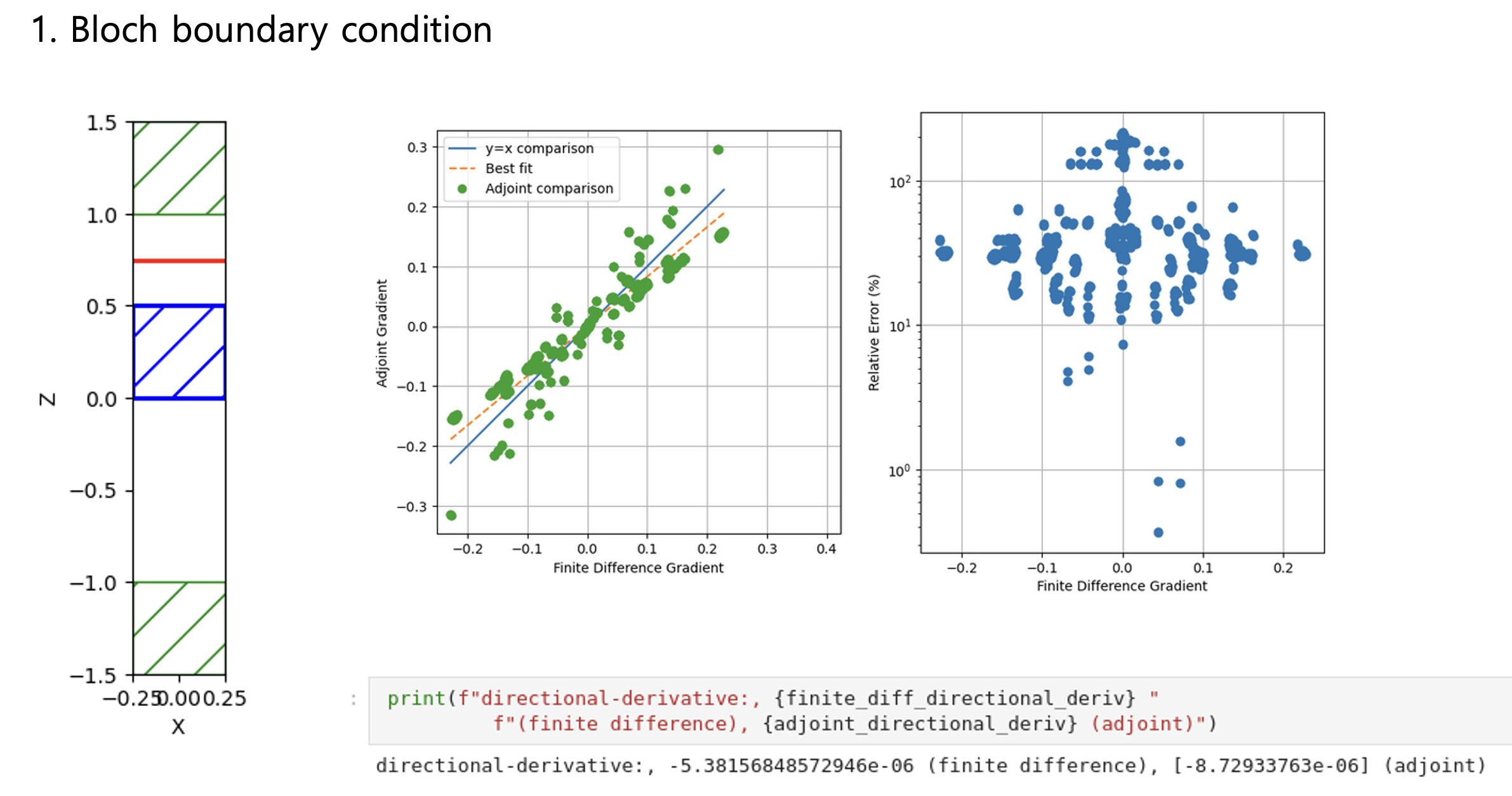
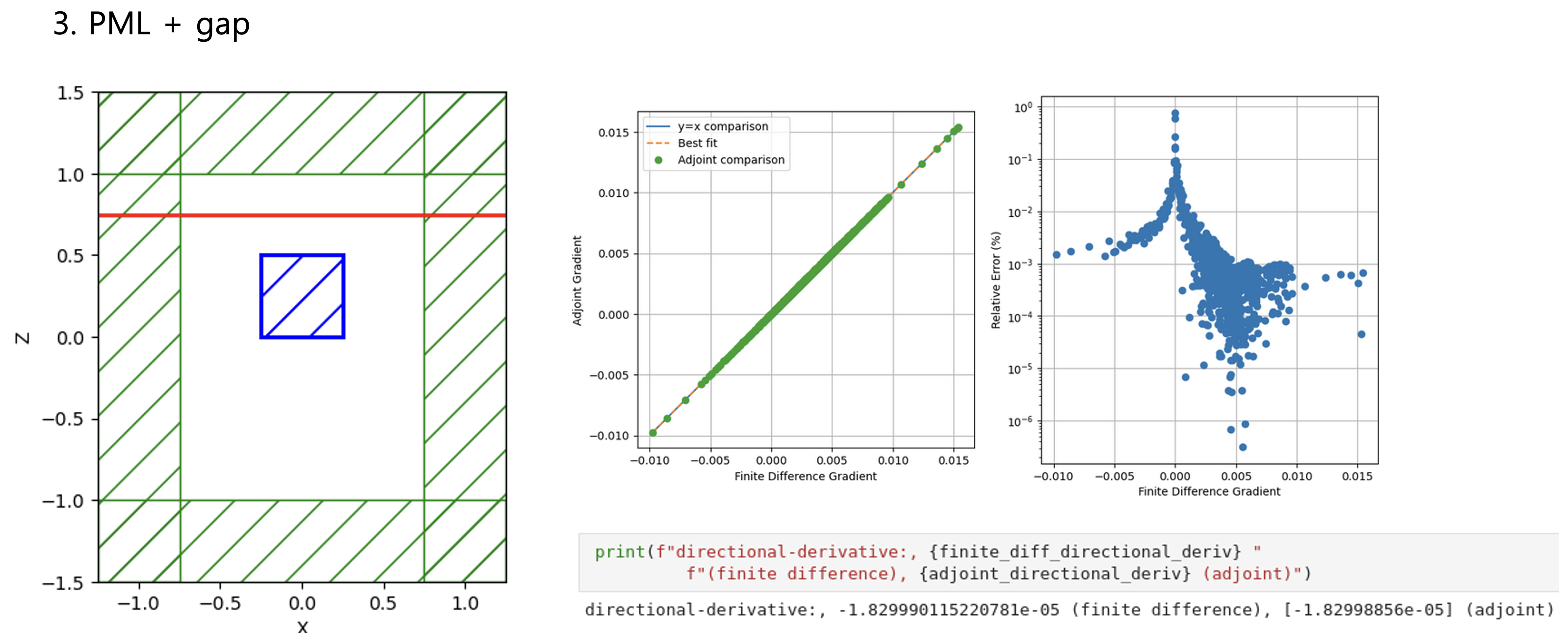
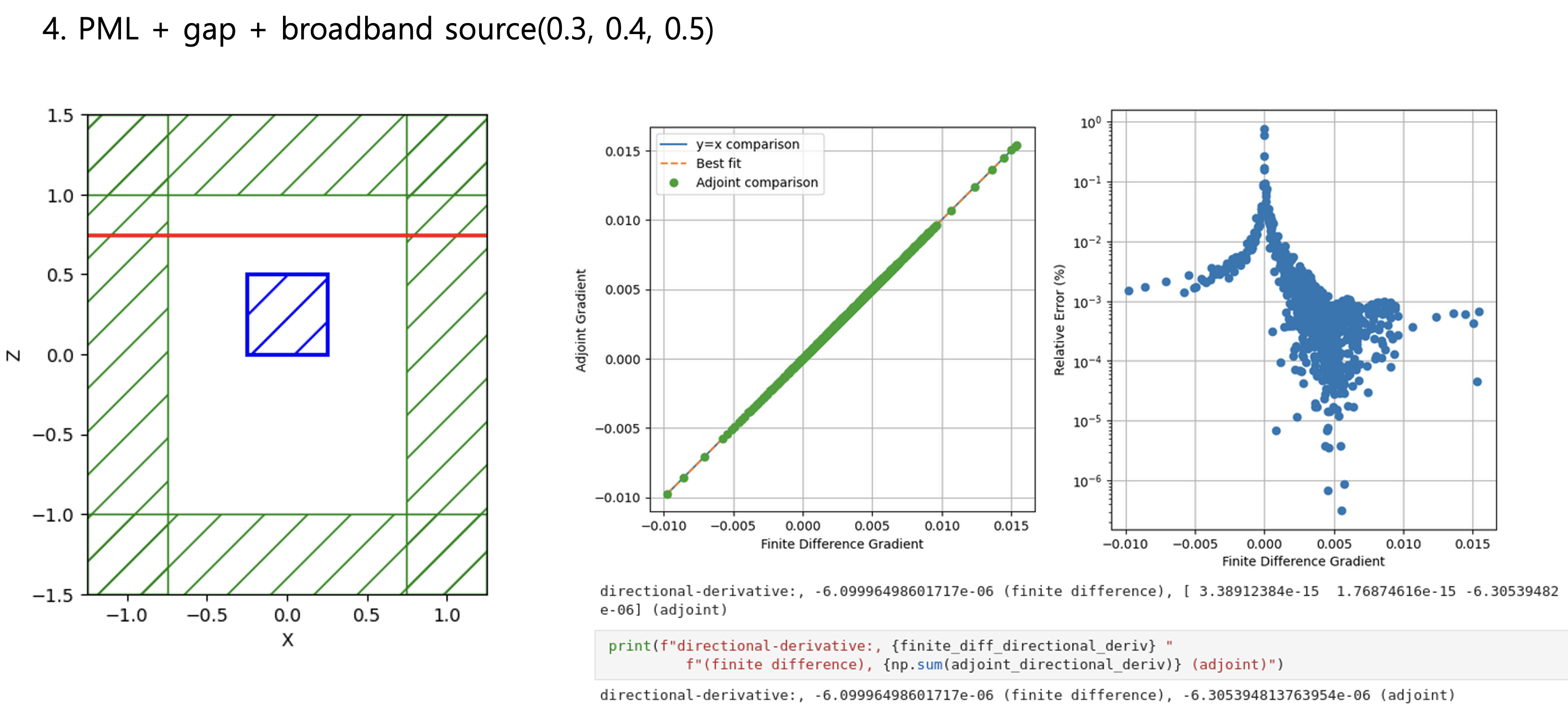
Python Meep: 3D adjoint gradient accuracy issue

Hello all,
I'm testing a smaller 3D toy problem, but I still need help with the adjoint gradient accuracy issue using the Bloch boundary.

When I set all boundaries with PML, the accuracy of the adjoint gradient in 3D is correct.
However, when using the Bloch boundary demonstrated in Fig. 1, the error of the adjoint gradient is high.

Fig 1

  • Fig.1 Bloch boundary condition

Fig 2

  • Fig.2 PML boundary condition

Fig 3

  • Fig. 3 PML with design region gap

Fig 4

  • Fig. 4 PML with design region gap + broadband source

Considering Fig. 1 ~ 4 results, the more unrelated the design region is to the boundary conditions, the more accurately the adjoint gradient is measured.
In other words, my toy problem concludes that Adjoint simulation works well but does not match when I have Bloch boundary conditions.

Do you have any workarounds for these issues, or can you comment?
If you have any suggestions or if there's something you'd like me to test in your source code, I'm more than willing to assist.


Toy problem code - Bloch boundary condition
"""Validates the adjoint gradient of a metalens in 3d."""

import meep as mp
import meep.adjoint as mpa
import numpy as np
from autograd import numpy as npa
from matplotlib import pyplot as plt

Air = mp.Medium(index=1.0)
SiN = mp.Medium(index=1.5)


resolution = 20 
Lpml = 0.5 
pml_layers = [mp.PML(thickness = Lpml, direction = mp.Z)]
Sourcespace = 0.5

design_region_width_x = 0.5
design_region_width_y = 0.5 
design_region_height = 0.5 

Sx = design_region_width_x
Sy = design_region_width_y
Sz = Lpml + design_region_height + Sourcespace + 1 + Lpml
cell_size = mp.Vector3(Sx, Sy, Sz)

wavelengths = np.array([0.5])
frequencies = 1/wavelengths
nf = len(frequencies) 

design_region_resolution = int(resolution)

fcen = 1 / 0.5
width = 0.1
fwidth = width * fcen

source_center = [0, 0, Sz / 2 - Lpml - Sourcespace / 2 ] 
source_size = mp.Vector3(Sx, Sy, 0)
src = mp.GaussianSource(frequency=fcen, fwidth=fwidth)
source = [mp.Source(src, component=mp.Ex, size=source_size, center=source_center,),]

Nx = int(round(design_region_resolution * design_region_width_x)) 
Ny = int(round(design_region_resolution * design_region_width_y)) 
Nz = int(round(design_region_resolution * design_region_height))

design_variables = mp.MaterialGrid(mp.Vector3(Nx, Ny, Nz), Air, SiN, grid_type="U_MEAN",do_averaging=False)
design_region = mpa.DesignRegion(
    design_variables,
    volume=mp.Volume(
        center=mp.Vector3(0, 0, Sz / 2 - Lpml - Sourcespace - design_region_height/2),
        size=mp.Vector3(design_region_width_x, design_region_width_y, design_region_height),
    ),
)

geometry = [
    mp.Block(
        center=design_region.center, size=design_region.size, material=design_variables
    ),
]

sim = mp.Simulation(
    cell_size=cell_size, 
    boundary_layers=pml_layers,
    geometry=geometry,
    sources=source,
    default_material=Air, 
    resolution=resolution,
    k_point = mp.Vector3(0,0,0)
)

monitor_position_0, monitor_size_0 = mp.Vector3(-design_region_width_x/2, design_region_width_y/2, -Sz/2 + Lpml + 0.5/resolution), mp.Vector3(0.01,0.01,0) 

FourierFields_0_x = mpa.FourierFields(sim,mp.Volume(center=monitor_position_0,size=monitor_size_0),mp.Ex,yee_grid=True)


ob_list = [FourierFields_0_x]


def J(fields):
    return npa.mean(npa.abs(fields[:,1]) ** 2)

opt = mpa.OptimizationProblem(
    simulation=sim,
    objective_functions=[J],
    objective_arguments=ob_list,
    design_regions=[design_region],
    frequencies=frequencies,
    decay_by=1e-5,
)

f0, dJ_du = opt()

db = 1e-5
choose = 1000
g_discrete, idx = opt.calculate_fd_gradient(num_gradients=choose, db=db)

(m, b) = np.polyfit(np.squeeze(g_discrete), dJ_du[idx], 1)

min_g = np.min(g_discrete)
max_g = np.max(g_discrete)

fig = plt.figure(figsize=(12, 6))

plt.subplot(1, 2, 1)
plt.plot([min_g, max_g], [min_g, max_g], label="y=x comparison")
plt.plot([min_g, max_g], [m * min_g + b, m * max_g + b], "--", label="Best fit")
plt.plot(g_discrete, dJ_du[idx], "o", label="Adjoint comparison")
plt.xlabel("Finite Difference Gradient")
plt.ylabel("Adjoint Gradient")
plt.legend()
plt.grid(True)
plt.axis("square")

plt.subplot(1, 2, 2)
rel_err = (
    np.abs(np.squeeze(g_discrete) - np.squeeze(dJ_du[idx]))
    / np.abs(np.squeeze(g_discrete))
    * 100
)
plt.semilogy(g_discrete, rel_err, "o")
plt.grid(True)
plt.xlabel("Finite Difference Gradient")
plt.ylabel("Relative Error (%)")
plt.show()

plt.savefig("graph.png")
plt.cla()  
plt.clf()  
plt.close() 
plt.show()

Checked comment and issue list before upload this issue.
  • Try swapping your PML out for absorbers.
  • Maybe make them a bit larger (do some convergence checks) and remove the maximum_runtime limit
  • Regarding the parameters in your test script, I would use a larger resolution (30), smaller finite difference size (~1e-7), and longer maximum_run_time (500 or 1000).
  • The gradients shouldn't really be sensitive to resolution anymore.
  • updated script with suggestion to disable subpixel smoothing in MaterialGrid (on by default) from @smartalecH which significantly improves accuracy.

Sign up for free to join this conversation on GitHub. Already have an account? Sign in to comment
Projects
None yet
Development

No branches or pull requests

4 participants