
Topological data analysis(TDA) is potential to find better representation of the data specially the shape of data. TDA can visualize the high dimensional data and characterize the intrinsic invariants of the data. It is close to computational geometry, manifold learning and computational topology. It is one kind of descriptive representation learning.
Problems of data analysis share many features with these two fundamental integration tasks: (1) how does one infer high dimensional structure from low dimensional representations; and (2) how does one assemble discrete points into global structure.
As The NIPS 2012 workshop on Algebraic Topology and Machine Learning puts:
Topological methods and machine learning have long enjoyed fruitful interactions as evidenced by popular algorithms like
ISOMAP, LLE and Laplacian Eigenmapswhich have been borne out of studying point cloud data through the lens of geometry. More recently several researchers have been attempting to also understand the algebraic topological properties of data. Algebraic topology is a branch of mathematics which uses tools from abstract algebra to study and classify topological spaces. The machine learning community thus far has focused almost exclusively on clustering as the main tool for unsupervised data analysis. Clustering however only scratches the surface, and algebraic topological methods aim at extracting much richer topological information from data.


Topological Data Analysis as its name shown takes the advantages of topological properties of data, which makes it different from manifold learning or computational geometry.
- https://www.wikiwand.com/en/Topological_data_analysis
- Centre for Topological Data Analysis
- TDA overview
- Topological Data Analysis
- Topology-Based Active Learning
- The NIPS 2012 workshop on Algebraic Topology and Machine Learning.
- Topological Data Analysis - Part 4 - Persistent Homology
- Topological Methods in Data Analysis and Visualization @springer
- https://jsseely.github.io/notes/TDA/
- Applied topology
- WORKSHOP ON TOPOLOGY AND NEUROSCIENCE
- https://www.h-its.org/event/workshop-grg-2018/
- Dragon Applied Topology Conference
- Computational & Algorithmic Topology, Sydney
- Oxford Topology
- Computational Topology and Geometry: G22.3033.007 & G63.2400, Fall 2006
- Computational Topology and Geometry (CompTaG)
- Topological Methods for Machine Learning: An ICML 2014 Workshop in Beijing, China
- Towards topological machine learning
- Geometry and Topology of Data @ICERM
- Geometry and Learning from Data in 3D and Beyond @IPAM
- Topological Data Analysis: theory, examples, applications
- http://chomp.rutgers.edu/
- http://chomp.rutgers.edu/Projects/Topological_Data_Analysis.html
- https://www.jstage.jst.go.jp/article/tjsai/32/3/32_D-G72/_pdf
- https://scikit-tda.org/
- https://people.maths.ox.ac.uk/tillmann/TDA2019.html
- http://dauns.math.tulane.edu/~mathweb/clifford2012/
- https://www.researchgate.net/profile/Genki_Kusano
- https://www.researchgate.net/profile/Yasuaki_Hiraoka
One of the key messages around topological data analysis is that data has shape and the shape matters.
The shape is always not in the term of probability distribution function or cumulant distribution function.
The basic goal of TDA is to apply topology, one of the major branches of mathematics, to develop tools for studying geometric features of data.
Perhaps the most elegant demonstration of the dangers of summary statistics is Anscombe’s Quartet. It’s a group of four datasets that appear to be similar when using typical summary statistics, yet tell four different stories when graphed. Each dataset consists of eleven

As shown above, the shape matters. And the distribution can not tell us all the information the datasets encode.
Specially in high dimensional space, it is not easy to depict the shape of data sets in the term of probability distribution function and it is almost impossible to visualize or graph them without dimension reduction.
Capturing all kinds of shape requires different method algebraically.
Topology is and Effective Language to Describe Abstractions of Features from Raw Data.
- http://cscads.rice.edu/2012_CSCADS_pascucci_2.pdf
- http://cscads.rice.edu/index.htm
- http://www.math.zju.edu.cn/redir.php?catalog_id=22&object_id=60501
- http://xlim-sic.labo.univ-poitiers.fr/jerboa/
- http://www.sfu.ca/siatclass/IAT355/Spring2014/
- http://www.cs.columbia.edu/~xie/
- http://www.csce.uark.edu/~xintaowu/
- https://www.math.vu.nl/~sbhulai/
- http://www.cedmav.org/
- http://www.hpcc.unical.it/hpc2012/
- http://knowescape.org/
- https://tdai.osu.edu/tripods-workshop/
Shape of Data:
- Normally defined in terms of a distance metric.
- Euclidean distance, Hamming, correlation distance, etc.
- Encodes similarity.
| Property |
|---|
| Coordinate Freeness |
| Deformation Invariance |
| Compressed Representation |
- Anscombe’s Quartet, and Why Summary Statistics Don’t Tell the Whole Story
- https://zhuanlan.zhihu.com/p/25547263
- http://www.matrix67.com/blog/archives/2308
- Why TDA works?
- Studying the Shape of Data Using Topology
- Towards a topological–geometrical theory of group equivariant non-expansive operators for data analysis and machine learning
- https://zenodo.org/record/3264851#.XYLmjDYzaM9
Topology focuses on the invariants with respect to continuous mapping. It pays more attention to the geometrical or discrete properties of the objects such as the number of circles or holes. It is not distance-based as much as differential geometry.
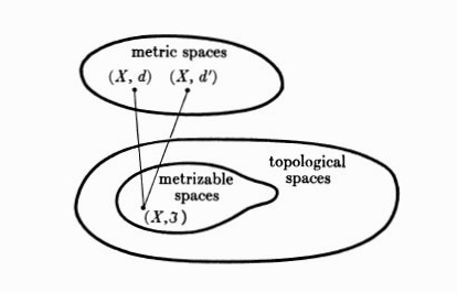
Definition: Let
$X$ be a non-empty set. A set$\tau$ of subsets of$X$ is said to be a topology if
$X$ and the empty set$\emptyset$ belong to$\tau$ ;- the union of any number of sets in
$\tau$ belongs to$\tau$ ;- the intersection of any two sets in
$\tau$ belongs to$\tau$ .
The pair
$(X,\tau)$ is called a topological space.
As the definition shows the topology may be really not based on the definition of distance or measure. The set can be countable or discountable.e3
Definition: Let
$(X,\tau)$ be a topological space. Then the members of$\tau$ (the subsets of$X$ ) is said to be open set. If$X-S$ is open set, we call$S$ as closed set.
From this definition, the open or close set is totally dependent on the set family
Like others in mathematics, the definition of topology is really abstract and strange like the outer space from the eyes of the ordinary living in the earth. Mathematics texts are almostly written in logic order and for the ideal cases. A good piece of news is that topological data analysis does provide many vivid example and concrete application, which does not only consist of mathematical concepts or theorems.
Definition A topological space
$(X, \tau)$ is said to be connected if$X$ is not the union of two disjoint nonempty open sets. Consequently, a topological space is disconnected if the union of any two disjoint nonempty subsets in$\tau$ produces$X$ .
Topological data analysis employs the use of simplicial complexes, which are complexes of geometric structures called simplices (singular: simplex). TDA uses simplicial complexes because they can approximate more complicated shapes and are much more mathematically and computationally tractable than the original shapes that they approximate.
Simplices are discrete building blocks for topological spaces.
For example, the probability simplex in
In fact, each component in probability simplex is in the interval
An n-simplex
$\sigma$ is the convex hull of$n + 1$ affinely ndependent vertices$S=$ Definition A k-simplex in$X$ is an unordered collection of$k + 1$ distinct elements of$X$ .
- Simplicial Complexes and Simplicial Homology
- http://ibykus.sdf.org/website/lang/de/algtop/
- https://simplicial.readthedocs.io/en/latest/simplicialcomplex.html
- simplicial: Simplicial topology in Python

The faces of a simplex are its boundaries.
Definition An
abstract simplexis any finite set of vertices.
Definition A
complexis a collection of multiple simplices.
Definition A
simplicial complex$\mathcal {K}$ is a set of simplices that satisfies the following conditions:
- Any face of a simplex in
$\mathcal {K}$ is also in$\mathcal {K}$ .- The intersection of any two simplices
$\sigma_{1}, \sigma_{2}\in \mathcal {K}$ is either$\emptyset$ or a face of both$\sigma_{1}$ and$\sigma_{2}$ .
Definition (Vietoris-Rips Complex) If we have a set of points
$P$ of dimension$d$ , and$P$ is a subset of$R^d$ , then the Vietoris-Rips (VR) complex$V_{\epsilon}(P)$ at scale$\epsilon$ (the VR complex over the point cloud$P$ with parameter$\epsilon$ ) is defined as: $$ V_{\epsilon}(P) = {\sigma\subset P\mid d(u, v)\leq \epsilon,\forall u≠v\in\sigma} $$
These VR complexes have been used as a way of associating a simplicial complex to point cloud data sets.
-
Flag/clique complexes : Given a graph (network)
$X$ , the flag complex or clique complex of$X$ is the maximal simplicial complex$X$ that has the graph as its 1-skeleton:$X^{(1)}=X$ . -
Banner Complexes: From flag complexes to banner complexes
-
Nerve Complexes: Nerves Let
$X$ be a topological space and $U = {U_{\alpha}}{\alpha\in A}$ a covering of $X$. The nerve of $U$, denoted $N(U)$, is the abstract simplicial complex with vertex set $A$ and where ${\alpha_0, \cdots , \alpha_k }$ spans a k-simplex if and only if $$U{\alpha_0}\cap\cdots\cap U_{\alpha_k}\not=\emptyset.$$ -
Dowker Complexes: For simplicity, let
$X$ and$Y$ be finite sets with #R \subset X\times Y$ representing the ones in a binary matrix (also denoted R) whose columns are indexed by$X$ and whose rows are indexed by$Y$ . TheDowker complexof$R$ on$X$ is the simplicial complex on the vertex set$X$ defined by the rows of the matrix$R$ . That is, each row of$R$ determines a subset of$X$ : use these to generate a simplex and all its faces. Doing so for all the rows gives the Dowker complex on$X$ . There is a dual Dowker complex on$Y$ whose simplices on the vertex set$Y$ are determined by the ones in columns of$R$ . -
Cell Complexes: Cell Complexes: Definitions
https://ncatlab.org/nlab/show/CW+complex
Nerve Theorem
Definition A family
$\Delta$ of non-empty finite subsets of a set$S$ is anabstract simplicial complexif, for every set$X$ in$\Delta$ , and every non-empty subset$Y \subset X$ ,$Y$ also belongs to$\Delta$ .
Definition The
n-chain, denoted$C_n(S)$ is the subset of an oriented abstract simplicial complex$S$ of n-dimensional simplicies.
Definition The
boundaryof an n-simplex$X$ with vertex set$[v_0, v_1, v_2,...v_n]$ , denoted$\partial(X)$ , is:$$\partial(X)=\sum_{i=0}^{n}(−1)^i[v_0, v_1, v_2,...v_n],$$ where the i-th vertex is removed from the sequence.
Persistent homology (henceforth just PH) gives us a way to find interesting patterns in data without having to "downgrade" the data in anyway so we can see it.
Robert Ghrist said that
Homology is the simplest, general, computable invariant of topological data. In its most primal manifestation, the homology of a space
$X$ returns a sequence of vector spaces$H•(X)$ , the dimensions of which count various types of linearly independent holes in$X$ . Homology is inherently linear-algebraic, but transcends linear algebra, serving as the inspiration for homological algebra. It is this algebraic engine that powers the subject.
Definition A
homotopybetween maps,$f_0 \simeq f_1 : X \to Y$ is a continuous 1-parameter family of maps$f_t: X \to Y$ . Ahomotopy equivalenceis a map$f : X \to Y$ with a homotopy inverse,$g: Y \to X$ satisfying$f \circ g \simeq {Id}_Y$ and$g \circ f \simeq {Id}_X$ .


Euler Characteristic
- http://outlace.com/TDApart1.html
- http://outlace.com/TDApart2.html
- http://outlace.com/TDApart3.html
- http://outlace.com/TDApart4.html
- http://outlace.com/TDApart5.html
- Homological Algebra and Data by Robert Ghrist
- homotopy theory
- Henry Adams: Persistent Homology
- https://www.wikiwand.com/en/Topology
- Topology Without Tears by Sidney A. Morris
- Geometric Topology
- Relationships, Geometry, and Artificial Intelligence
Topological data analysis as one data processing method is selected topic for some students on computer science and applied mathematics. It is not popular for the statisticians, where there is no estimation and test.
Topological data analysis (TDA) refers to statistical methods that find structure in data. As the name suggests, these methods make use of topological ideas. Often, the term TDA is used narrowly to describe a particular method called persistent homology.
TDA, which originates from mathematical topology, is a discipline that studies shape. It’s concerned with measuring the shape, by means applying math functions to data, and with representing it in forms of topological networks or combinatorial graphs.
Topological data analysis is more fundamental than revolutionary: such methods are not intended to supplant analytic, probabilistic, or spectral techniques. They can however reveal a deeper basis for why some data sets and systems behave the way they do. It is unwise to wield topological techniques in isolation, assuming that the weapons of unfamiliar "higher" mathematics are clad in incorruptible silver
There is another field that deals with the topological and geometric structure of data: computational geometry. The main difference is that in TDA we treat the data as random points, whereas in computational geometry the data are usually seen as fixed.

TDA can be applied to manifold estimation, nonlinear dimension reduction, mode estimation, ridge estimation and persistent homology.
- IDAC TDA Workshop: Topological Data Analysis for Discovery in Multi-scalar Biomedical Data – Applications in Musculoskeletal Imaging
- International Workshop on Topological Data Analysis in Biomedicine (TDA-Bio) Seattle, WA, October 2, 2016
- Deep Learning with Topological Signatures - Persistent Homology and Machine Learning
- Topological data analysis for imaging and machine learning
- Time Series Featurization via Topological Data Analysis
- Topological Analysis and Visualization of Cyclical Behavior in Memory Reference Traces
- http://tdaphenomics.eecs.wsu.edu/
- https://wasp-sweden.org/topological-data-analysis/
- http://unboxai.org/
- Topological Data Analysis and Persistent Homology
- An Introduction to Topological Data Analysis for Physicists: From LGM to FRBs
Topological analysis using persistent homology
- Finds topological invariants in data (# of connected components, enclosed voids, etc.)
- Input: a (density) function,
$f$ - Output: topological structures & their persistence
- Def: given threshold
$t$ , the superlevel set$f^{-1}(t)={x\mid f(x)\geq t}$ .- the true structures are hidden in superlevel sets
- consider the whole stack of superlevel sets
- identify structures that often appear (high persistence)
- Output: persistence diagram – dots representing all structures
- http://www.sci.utah.edu/~beiwang/acmbcbworkshop2016/slides/ChaoChen.pdf
- BARCODES: THE PERSISTENT TOPOLOGY OF DATA
- Apply a filter function to project data onto a lower dimensional space
- Performs partial clustering in the level sets
Mapper is an important tool used in TDA for data visualization.
- Input
- point cloud;
- “filter function;”
- covering of a metric space;
- clustering algorithm;
- various other parameters.
- Output
- Graph (or higher simplicial complex) which is thought to capture aspects of the topology of the point cloud.
- The Mapper Algorithm Western TDA Learning Seminar
- Topology ToolKit: Efficient, generic and easy Topological data analysis and visualization
- Data Visualization with TDA Mapper, Spring 2018
- http://danifold.net/mapper/
- https://github.com/scikit-tda/kepler-mapper
- https://www.ayasdi.com/
- Extracting insights from the shape of complex data using topology.
- Topological Methods for the Analysis of High Dimensional Data Sets and 3D Object Recognition
- https://zhuanlan.zhihu.com/p/31734839
- Interesting Paths in the Mapper
- A header only software library helps to visually discover the insights of high dimensional complex data set.
- Toward A Scalable Exploratory Framework for Complex High-Dimensional Phenomics Data
- Machine Learning Explanations with Topological Data Analysis
Dr Vitaliy Kurlin Applied Algebraic Topology (AAT) network in the UK
Wang Bei was a PI of DBI: ABI Innovation: A Scalable Framework for Visual Exploration and Hypotheses Extraction of Phenomics Data using Topological Analytics.

- CSIC 5011: Topological and Geometric Data Reduction and Visualization Fall 2019
- https://geometry.stanford.edu/member/guibas/
- https://math.berkeley.edu/~smale/
- https://yao-lab.github.io/
- A series of blogs on TDA
- Topological Data Analysis @ Annual Review of Statistics and Its Application
- Topological Data Analysis by peterbubenik
- Applied Algebraic Topology Research Network
- Henry Adams interests in computational topology and geometry, combinatorial topology, and applied topology
- Robert Ghrist's research is in applied topology that is, applications of topology to engineering systems, data, dynamics, & more
- CSE 5559: Computational Topology and Data Analysis by Tamal K Dey
- CMU TopStat
- Topological & Functional Data Analysis @ CMU
- Topological Data Analysis: an Overview of the World’s Most Promising Data Mining Methodology
- Index of /~beiwang/teaching/cs6170-spring-2017
- Topological Data Analysis: One Applied Mathematician’s Heartwarming Story of Struggle, Triumph, and (Ultimately) More Struggle By Chad Topaz
- Scalable topological data analysis
- Topology, Computation and Data Analysis
- Topological Data Analysis Learning Seminar, Summer 2018
- https://www-apr.lip6.fr/~tierny/topologicalDataAnalysisClass.html
- Topological Data Analysis and Persistent Homology
- http://www.columbia.edu/~jss2219/tda/
- https://github.com/henryadams/Charleston-TDA-ML
- https://github.com/prokopevaleksey/TDAforCNN
- https://github.com/ognis1205/spark-tda
- https://github.com/stephenhky/PyTDA
- http://www.columbia.edu/~jss2219/tda/Resources.html
- Open Source Software for TDA
- https://www.giotto.ai/
- https://pypi.org/project/giotto-learn/
- https://heig-vd.ch/en/research/reds
- https://www.l2f.ch/
- https://www.epfl.ch/labs/hessbellwald-lab/
- https://github.com/giotto-ai/giotto-learn
- https://giotto.readthedocs.io/en/latest/index.html
- https://docs.giotto.ai/
- http://tdaphenomics.eecs.wsu.edu/
- Topological Data Analysis of fMRI data:11 Apr 2018 by Manish Saggar
- Topological Data Analysis for Genomics and Applications to Cancer
- Topological Data Analysis and Machine Learning for Classifying Atmospheric River Patterns in Large Climate Datasets
- DBI: ABI Innovation: A Scalable Framework for Visual Exploration and Hypotheses Extraction of Phenomics Data using Topological Analytics
- Algebraic topology and neuroscience: a bibliography
- Mass Cytometry and Topological Data Analysis Reveal Immune Parameters Associated with Complications after Allogeneic Stem Cell Transplantation
- Two Applications of Topological Methods for Neuronal Morphology Analysis
- Utilizing Topological Data Analysis to Detect Periodicity
- Topological Problems in Molecular Biology, American Mathematical Society Central Section
- A survey of Topological Data Analysis Methods for Big Data in Healthcare Intelligence
Computational topology is the mathematical theoretic foundation of topological data analysis. It is different from the deep neural network that origins from the engineering or the simulation to biological neural network. Topological data analysis is principle-driven and application-inspired in some sense.
CS 598: Computational Topology Spring 2013 covers the following topics:
Potential mathematical topics include the topology of cell complexes, topological graph theory, homotopy, covering spaces, simplicial homology, persistent homology, discrete Morse theory, discrete differential geometry, and normal surface theory. Potential computing topics include algorithms for computing topological invariants, graphics and geometry processing, mesh generation, curve and surface reconstruction, VLSI routing, motion planning, manifold learning, clustering, image processing, and combinatorial optimization.

- Computational Algebraic Topology
- https://datawarrior.wordpress.com/
- http://people.maths.ox.ac.uk/tillmann/CAT.html
- Theory and Algorithms in Data Science
- http://graphics.stanford.edu/courses/cs468-09-fall/
- CS 468 - Fall 2002: Introduction to Computational Topology
- http://people.maths.ox.ac.uk/nanda/source/RSVWeb.pdf
- The Čech Complex and the Vietoris-Rips Complex
- CS 598: Computational Topology , Spring 2013, Jeff Erickson
- INF556 -- Topological Data Analysis (2018-19) Steve Oudot
- SF2956 Topological Data Analysis 7.5 credits
- Computational Topology and Geometry G22.3033.007 & G63.2400, Fall 2006 @NYU
- C3.9 Computational Algebraic Topology (2016-2017)
- CPS296.1: COMPUTATIONAL TOPOLOGY @Duke
- Math 574--Introduction to Computational Topology (Spring 2016)
- NSF-CBMS Conference and Software Day on Topological Methods in Machine Learning and Artificial Intelligence: May 13–17 and May 18, 2019. Department of Mathematics, College of Charleston, South Carolina
- Data science and applied topology
- Machine Learning Explanations with Topological Data Analysis
- Topological Data Analysis and Machine Learning Theory
- https://ima.umn.edu/2013-2014/


https://shapeofdata.wordpress.com/
Computational geometry uses some information of samples or local information of the geometrical objects to reconstruct/describe the whole object.
In computer vision, the task 3D reconstruction is a typical example of computational geometry.
- Probabilistic Approach to Geometry
- Applied Geometry Lab @Caltech
- Titane: Geometric Modeling of 3D Environments
- Computational Geometry and Modeling G22.3033.007 Spring 2005
- Multi-Res Modeling Group@Caltech
- Geometry in Graphics Group in Computer Science and Engineering@Michigan State University
- Computational Geometry Week (CG Week) 2019
- Computational Geometry and Topology
- http://www.computational-geometry.org/
- Handbook of Discrete and Computational Geometry —Third Edition— edited by Jacob E. Goodman, Joseph O'Rourke, and Csaba D. Tóth
- http://brickisland.net/DDGSpring2016/2016/01/22/reading-3-topological-data-analysis/
- http://graphics.stanford.edu/courses/cs468-14-winter/
- https://drona.csa.iisc.ac.in/~gsat/Course/CGT/
- http://www.computational-geometry.org/
- https://project.inria.fr/gudhi/
- http://web.cse.ohio-state.edu/~wang.1016/courses/788/
- Higher Dimensional Geometry Understanding
http://cs233.stanford.ed https://tgda.osu.edu/
Geometric Data Analysis and topological data analysis are out of the mainstream of quantitative statistics while the quantity also matters in geometric data analysis.
In conventional statistics, the core concepts are distribution (count in brief) and in/dependence, which is regarded as the reverse engineer of the probability theory. It is supposed that the data is embedded in some "flat" subspace in
- GEOMETRIC DATA ANALYSIS, U CHICAGO, MAY 20-23 2019
- Geometric Data Analysis Reading Group
- Foundations of Geometric Methods in Data Analysis
- CS233 Class Schedule for Spring Quarter '17-'18
- MA500 Geometric Foundations of Data Analysis
- Special Session on Geometric Data Analysis
- Workshop - Statistics for geometric data and applications to anthropology
- CSIC 5011: Topological and Geometric Data Reduction and Visualization
- 4th conference on Geometric Science of Information
- Geometric Image Processing @ Department of Computer Science Technion - Israel Institute of Technology

- The geometry of optimal transportation
- Transformations of PDEs: Optimal Transport and Conservation Laws by Woo-Hyun Cook
- Optimal transport, old and new
- Math 3015 (Topics in Optimal Transport). Spring 2010
- https://optimaltransport.github.io/
- http://www.math.ucla.edu/~wgangbo/Cedric-Villani.pdf
- https://pot.readthedocs.io/en/stable/
- Optimal Transport @ESI
- Optimal Transport Methods in Density Functional Theory (19w5035)
- Discrete OT
- Optimal Transport & Machine Learning
- Optimal Transport and Machine learning course at DS3 2018
- Hot Topics: Optimal transport and applications to machine learning and statistics
- An intuitive guide to optimal transport for machine learning
- http://faculty.virginia.edu/rohde/transport/
- http://otml17.marcocuturi.net/
- https://anr.fr/Project-ANR-17-CE23-0012
- http://otnm.lakecomoschool.org/program/
- https://sites.uclouvain.be/socn/drupal/socn/node/113
- Topics on Optimal Transport in Machine Learning and Shape Analysis(OT.ML.SA)
- Optimal Transport in Biomedical Imaging
- Optimal transport for documents classification: Classifying news with Word Mover Distance
- Monge-Kantorovich Optimal Transport – Theory and Applications