- Content
- Regression Analysis
- Machine Learning
Regression is a method for studying the relationship between a response variable
Regression is not function fitting. In function fitting, it is well-defined -
Linear regression is the "hello world" in statistical learning. It is the simplest model to fit the datum. We will induce it in the maximum likelihood estimation perspective. See this link for more information https://www.wikiwand.com/en/Regression_analysis.
A linear regression model assumes that the regression function
By convention (very important!):
-
$\mathrm{x}$ is assumed to be standardized (mean 0, unit variance); -
$\mathrm{y}$ is assumed to be centered.
For the linear regression, we could assume
The likelihood of the errors are
$$
L(\epsilon_1,\epsilon_2,\cdots,\epsilon_n)=\prod_{i=1}^{n}\frac{1}{\sqrt{2\pi}}e^{-\epsilon_i^2}.
$$
In MLE, we have shown that it is equivalent to $$ \arg\max \prod_{i=1}^{n}\frac{1}{\sqrt{2\pi}}e^{-\epsilon_i^2}=\arg\min\sum_{i=1}^{n}\epsilon_i^2=\arg\min\sum_{i=1}^{n}(y_i-f(x_i))^2. $$
| Linear Regression and Likelihood Maximum Estimation |
|---|
 |
For linear regression, the function
- the residual error
${\epsilon_i}_{i=1}^{n}$ are i.i.d. in Gaussian distribution; - the inverse matrix
$(X^{T}X)^{-1}$ may not exist in some extreme case.
See more on Wikipedia page.
When the matrix
In the perspective of computation, we would like to consider the regularization technique; In the perspective of Bayesian statistics, we would like to consider more proper prior distribution of the parameters.
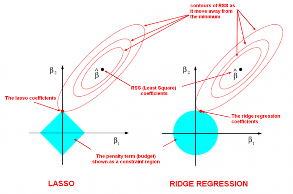
It is to optimize the following objective function with parameter norm penalty
$$
PRSS_{\ell_2}=\sum_{i=1}^{n}(y_i-w^Tx_i)^2+\lambda w^{T}w=|Y-Xw|^2+\lambda|w|^2,\tag {Ridge}.
$$
It is called penalized residual sum of squares.
Taking derivatives, we solve
$$
\frac{\partial PRSS_{\ell_2}}{\partial w}=2X^T(Y-Xw)+2\lambda w=0
$$
and we gain that
$$
w=(X^{T}X+\lambda I)^{-1}X^{T}Y
$$
where it is trackable if
LASSO is the abbreviation of Least Absolute Shrinkage and Selection Operator.
-
It is to minimize the following objective function: $$ PRSS_{\ell_1}=\sum_{i=1}^{n}(y_i-w^Tx_i)^2+\lambda{|w|}_{1} =|Y-Xw|^2+\lambda{|w|}_1,\tag {LASSO}. $$
-
the optimization form: $$ \begin{align} \arg\min_{w}\sum_{i=1}^{n}(y_i-w^Tx_i)^2 &\qquad\text{Objective function} \ \text{subject to},{|w|}_1 \leq t &\qquad\text{constraint}. \end{align} $$
-
the selection form: $$ \begin{align} \arg\min_{w}{|w|}1 \qquad &\text{Objective function} \ \text{subject to},\sum{i=1}^{n}(y_i-w^Tx_i)^2 \leq t \qquad &\text{constraint}. \end{align} $$ where ${|w|}1=\sum{i=1}^{n}|w_i|$ if
$w=(w_1,w_2,\cdots, w_n)^{T}$ .
More solutions to this optimization problem:
- Q&A in zhihu.com;
- ADMM to LASSO;
- Regularization: Ridge Regression and the LASSO;
- Least angle regression;
- http://web.stanford.edu/~hastie/StatLearnSparsity/
- 历史的角度来看,Robert Tibshirani 的 Lasso 到底是不是革命性的创新?- 若羽的回答 - 知乎
- http://www.cnblogs.com/xingshansi/p/6890048.html
| LASSO and Ridge Regression |
|---|
 |
| The LASSO Page ,Wikipedia page and Q&A in zhihu.com |
| More References in Chinese blog |
If we suppose the prior distribution of the parameters
When the sample size of training data
See more on http://web.stanford.edu/~hastie/TALKS/glmnet_webinar.pdf or http://www.princeton.edu/~yc5/ele538_math_data/lectures/model_selection.pdf.
We can deduce it by Bayesian estimation if we suppose the prior distribution of the parameters
See Bayesian lasso regression at http://faculty.chicagobooth.edu/workshops/econometrics/past/pdf/asp047v1.pdf.
In ordinary least squares, we assume that the errors ${{\epsilon}{i}}{i=1}^{n}$ are i.i.d. Gaussian, i.e.
Ordinary linear regression predicts the expected value of a given unknown quantity (the response variable, a random variable) as a linear combination of a set of observed values (predictors). This implies that a constant change in a predictor leads to a constant change in the response variable (i.e. a linear-response model). This is appropriate when the response variable has a normal distribution (intuitively, when a response variable can vary essentially indefinitely in either direction with no fixed "zero value", or more generally for any quantity that only varies by a relatively small amount, e.g. human heights).
However, these assumptions are inappropriate for some types of response variables. For example, in cases where the response variable is expected to be always positive and varying over a wide range, constant input changes lead to geometrically varying, rather than constantly varying, output changes. As an example, a prediction model might predict that 10 degree temperature decrease would lead to 1,000 fewer people visiting the beach is unlikely to generalize well over both small beaches (e.g. those where the expected attendance was 50 at a particular temperature) and large beaches (e.g. those where the expected attendance was 10,000 at a low temperature). The problem with this kind of prediction model would imply a temperature drop of 10 degrees would lead to 1,000 fewer people visiting the beach, a beach whose expected attendance was 50 at a higher temperature would now be predicted to have the impossible attendance value of −950. Logically, a more realistic model would instead predict a constant rate of increased beach attendance (e.g. an increase in 10 degrees leads to a doubling in beach attendance, and a drop in 10 degrees leads to a halving in attendance). Such a model is termed an exponential-response model (or log-linear model, since the logarithm of the response is predicted to vary linearly).
In a generalized linear model (GLM), each outcome
The GLM consists of three elements:
| Model components |
|---|
| 1. A probability distribution from the exponential family. |
| 2. A linear predictor |
| 3. A link function |
- https://xg1990.com/blog/archives/304
- https://zhuanlan.zhihu.com/p/22876460
- https://www.wikiwand.com/en/Generalized_linear_model
- Roadmap to generalized linear models in metacademy at (https://metacademy.org/graphs/concepts/generalized_linear_models#lfocus=generalized_linear_models)
- Course in Princeton
- Exponential distribution familiy
- 14.1 - The General Linear Mixed Model
The logistic distribution: $$ y\stackrel{\triangle}=P(Y=1|X=x)=\frac{1}{1+e^{-w^{T}x}}=\frac{e^{w^{T}x}}{1+e^{w^{T}x}} $$
where
i.e. $$ \log\frac{y}{1-y}=w^{T}x $$ in theory.
- https://www.wikiwand.com/en/Logistic_regression
- http://www.omidrouhani.com/research/logisticregression/html/logisticregression.htm
There is a section of projection pursuit and neural networks in Element of Statistical Learning.
Assume we have an input vector
where each parameter projection indices.
The function
The single index model in econometrics.
We seek the approximate minimizers of the error function $$ \sum_{n=1}^{N}[y_n - \sum_{m=1}^{M} g_m ( \left<\omega_m, x_i \right>)]^2 $$
over functions
And there is a PHD thesis Design and choice of projection indices in 1992.
- https://projecteuclid.org/euclid.aos/1176349519
- https://projecteuclid.org/euclid.aos/1176349520
- https://projecteuclid.org/euclid.aos/1176349535
- https://people.maths.bris.ac.uk/~magpn/Research/PP/PP.html
- https://www.wikiwand.com/en/Projection_pursuit_regression
- http://www.stat.cmu.edu/~larry/=stat401/
- http://cis.legacy.ics.tkk.fi/aapo/papers/IJCNN99_tutorialweb/node23.html
- https://www.pnas.org/content/115/37/9151
- https://www.ncbi.nlm.nih.gov/pubmed/30150379
- https://www.wikiwand.com/en/Additive_model
- https://www.wikiwand.com/en/Generalized_additive_model
- http://iacs-courses.seas.harvard.edu/courses/am207/blog/lecture-20.html
- Nonparametric regression https://www.wikiwand.com/en/Nonparametric_regression
- Multilevel model https://www.wikiwand.com/en/Multilevel_model
- A Tutorial on Bayesian Nonparametric Models
- Hierarchical generalized linear model https://www.wikiwand.com/en/Hierarchical_generalized_linear_model
- http://doingbayesiandataanalysis.blogspot.com/2012/11/shrinkage-in-multi-level-hierarchical.html
- https://twiecki.github.io/blog/2014/03/17/bayesian-glms-3/
- http://www.stat.cmu.edu/~larry/=sml
- http://www.stat.cmu.edu/~larry/
- http://www.stat.cmu.edu/~larry/=stat401/
- https://zhuanlan.zhihu.com/p/26830453

The goal of machine learning is to program computers to use example data or past experience to solve a given problem. Many successful applications of machine learning exist already, including systems that analyze past sales data to predict customer behavior, recognize faces or spoken speech, optimize robot behavior so that a task can be completed using minimum resources, and extract knowledge from bioinformatics data. From ALPAYDIN, Ethem, 2004. Introduction to Machine Learning. Cambridge, MA: The MIT Press..
- http://www.machine-learning.martinsewell.com/
- https://arogozhnikov.github.io/2016/04/28/demonstrations-for-ml-courses.html
- https://www.analyticsvidhya.com/blog/2016/09/most-active-data-scientists-free-books-notebooks-tutorials-on-github/
- https://data-flair.training/blogs/machine-learning-tutorials-home/
- https://github.com/ty4z2008/Qix/blob/master/dl.md
- https://machinelearningmastery.com/category/machine-learning-resources/
- https://machinelearningmastery.com/machine-learning-checklist/
- https://ml-cheatsheet.readthedocs.io/en/latest/index.html
- https://sgfin.github.io/learning-resources/
- https://cedar.buffalo.edu/~srihari/CSE574/index.html
- http://interpretable.ml/
- https://christophm.github.io/interpretable-ml-book/
- https://csml.princeton.edu/readinggroup
- https://www.seas.harvard.edu/courses/cs281/
- https://developers.google.com/machine-learning/guides/rules-of-ml/
- https://lilianweng.github.io/lil-log/2017/08/01/how-to-explain-the-prediction-of-a-machine-learning-model.html
- https://www.comp.nus.edu.sg/~reza/courses/cs6231/
There is another trichotomy in statistics
descriptive analysis, exploratory analysis, inferential analysis
The unsupervised and supervised learning
Unsupervised learning is a form of descriptive analytics. Predictive analytics aims to estimate outcomes from current data. Supervised learning is a kind of predictive analytics. Finally, prescriptive analytics guides actions to take in order to guarantee outcomes. Anomaly Detection Learning Resources
The most popular methods in statistics is maximum likelihood estimation. Density estimation can be classified to the parameter estimation in parametric setting.

It seems simple and easy while in fact it is not completely solved because of the diverse distributions.
For example, what is the probability density function of the pixels in the given size pictures?
Not all distribution function of interest are clear for us in high dimensional space although Gaussian mixture is a universal approximation of distribution function in
- stable distributions such as generalized Laplacian distribution in finance;
- semi-circle distribution of the random matrix eigenvalues in physics;
- sub-Gaussian distribution in high dimensional space.

And it is one of the core problems in statistical estimation. It is more difficult if we can not observe the samples directly such as the probability of root of polynomials given some properties. Like other tasks, the dimension curse makes it more complicated than in low dimensional space. Density estimation is related with sampling on random.
Parzen window is a non-parametric density estimation technique.
We firstly think the simple kernel function
- http://www.stat.cmu.edu/~larry/=sml/densityestimation.pdf
- https://cs.dartmouth.edu/wjarosz/publications/dissertation/appendixC.pdf
- http://assets.press.princeton.edu/chapters/s8355.pdf
- https://www.wikiwand.com/en/Tracy%E2%80%93Widom_distribution
- https://www.quantamagazine.org/beyond-the-bell-curve-a-new-universal-law-20141015/
https://www.wikiwand.com/en/Nonlinear_dimensionality_reduction https://www.cs.toronto.edu/~hinton/science.pdf
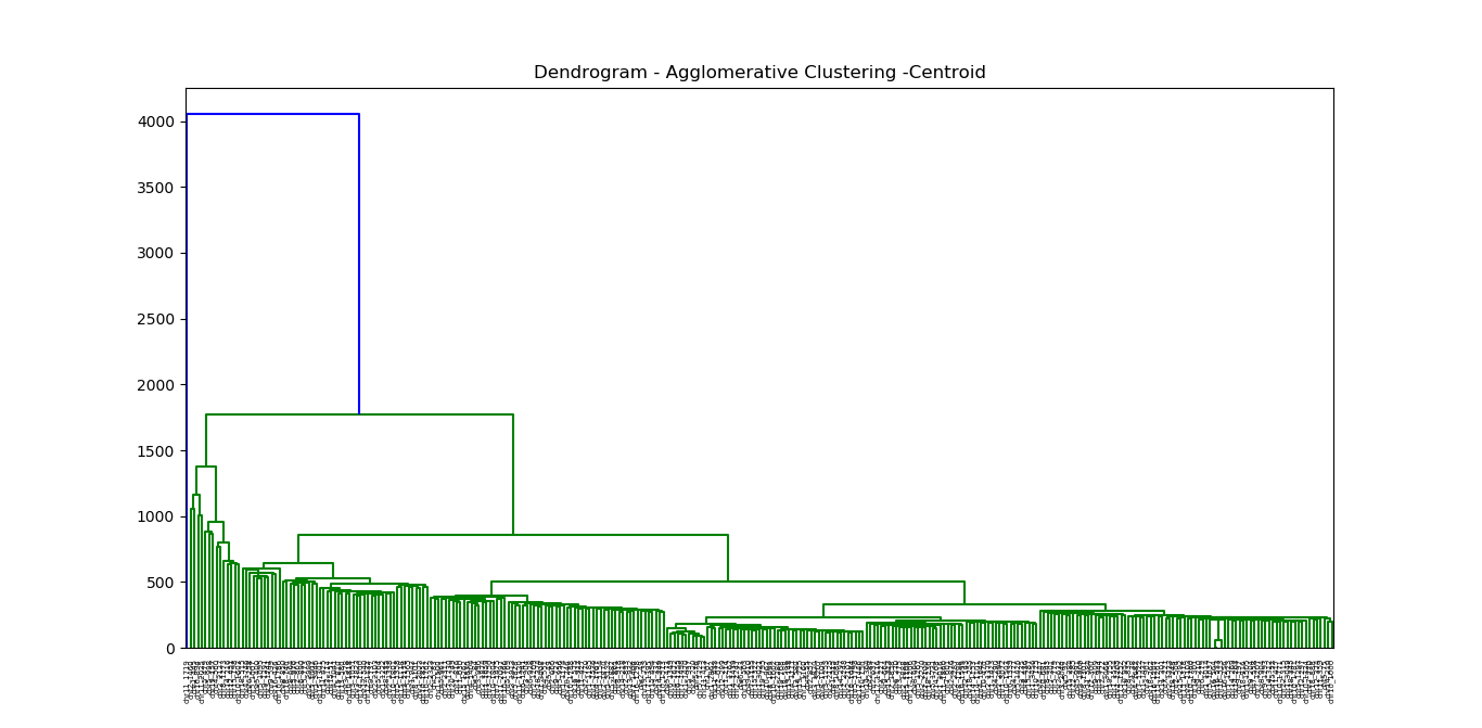
There are two different contexts in clustering, depending on how the entities to be clustered are organized.
In some cases one starts from an internal representation of each entity (typically an
The external representation of dissimilarity will be discussed in Graph Algorithm.
K-means is also called Lloyd’s algorithm.
- https://blog.csdn.net/qq_39388410/article/details/78240037
- http://iss.ices.utexas.edu/?p=projects/galois/benchmarks/agglomerative_clustering
- https://nlp.stanford.edu/IR-book/html/htmledition/hierarchical-agglomerative-clustering-1.html
- https://www.wikiwand.com/en/Hierarchical_clustering
- http://sklearn.apachecn.org/cn/0.19.0/modules/clustering.html
- https://www.wikiwand.com/en/Cluster_analysis
- https://www.toptal.com/machine-learning/clustering-algorithms
http://www.svms.org/history.html
http://www.svms.org/
http://web.stanford.edu/~hastie/TALKS/svm.pdf
http://bytesizebio.net/2014/02/05/support-vector-machines-explained-well/

- Kernel method at Wikipedia;
- http://www.kernel-machines.org/
- http://onlineprediction.net/?n=Main.KernelMethods
- https://arxiv.org/pdf/math/0701907.pdf
- http://disi.unitn.it/moschitti/Tree-Kernel.htm
- http://disi.unitn.it/moschitti/Kernel_Group.htm

Singular value decomposition is an extension of eigenvector decomposition of a matrix.
For the square matrix
Theorem: All eigenvalues of a symmetrical matrix are real.
Proof: Let
$A$ be a real symmetrical matrix and$Av=\lambda v$ . We want to show the eigenvalue$\lambda$ is real. Let$v^{\star}$ be conjugate transpose of$v$ .$v^{\star}Av=\lambda v^{\star}v,(1)$ . If$Av=\lambda v$ ,thus$(Av)^{\star}=(\lambda v)^{\star}$ , i.e.$v^{\star}A=\bar{\lambda}v^{\star}$ . We can infer that$v^{\star}Av=\bar{\lambda}v^{\star}v,(2)$ .By comparing the equation (1) and (2), we can obtain that$\lambda=\bar{\lambda}$ where$\bar{\lambda}$ is the conjugate of$\lambda$ .
Theorem: Every symmetrical matrix can be diagonalized.
See more at http://mathworld.wolfram.com/MatrixDiagonalization.html.
When the matrix is rectangle i.e. the number of columns and the number of rows are not equal, what is the counterpart of eigenvalues and eigenvectors?
Another question is if every matrix
Theorem: The matrix
$A$ and$B$ has the same eigenvalues except zero.Proof: We know that
$A=M_{m\times n}^TM_{m\times n}$ and$B=M_{m\times n}M_{m\times n}^T$ . Let$Av=\lambda v$ i.e.$M_{m\times n}^TM_{m\times n} v=\lambda v$ , which can be rewritten as$M_{m\times n}^T(M_{m\times n} v)=\lambda v,(1)$ , where$v\in\mathbb{R}^n$ . We multiply the matrix$M_{m\times n}$ in the left of both sides of equation (1), then we obtain$M_{m\times n}M_{m\times n}^T(M_{m\times n} v)=M_{m\times n}(\lambda v)=\lambda(M_{m\times n} v)$ .
Theorem: The matrix
$A$ and$B$ are non-negative definite, i.e.$\left<v,Av\right>\geq 0, \forall v\in\mathbb{R}^n$ and$\left<u,Bu\right>\geq 0, \forall u\in\mathbb{R}^m$ .Proof: It is
$\left<v,Av\right>=\left<v,M_{m\times n}^TM_{m\times n}v\right>=(Mv)^T(Mv)=|Mv|_2^2\geq 0$ as well as$B$ .
Theorem:
$M_{m\times n}=U_{m\times m}\Sigma_{m\times n} V_{n\times n}^T$ , where
$U_{m\times m}$ is an$m \times m$ orthogonal matrix;$\Sigma_{m\times n}$ is a diagonal$m \times n$ matrix with non-negative real numbers on the diagonal,$V_{n\times n}^T$ is the transpose of an$n \times n$ orthogonal matrix.
See the chapter Best-Fit Subspaces and Singular Value Decomposition (SVD) at https://www.cs.cornell.edu/jeh/book.pdf.
| SVD |
|---|
 |
See more at http://mathworld.wolfram.com/SingularValueDecomposition.html.
- http://www-users.math.umn.edu/~lerman/math5467/svd.pdf
- http://www.nytimes.com/2008/11/23/magazine/23Netflix-t.html
- https://zhuanlan.zhihu.com/p/36546367
- http://www.cnblogs.com/LeftNotEasy/archive/2011/01/19/svd-and-applications.html
- Singular value decomposition
- http://www.cnblogs.com/endlesscoding/p/10033527.html
- http://www.flickering.cn/%E6%95%B0%E5%AD%A6%E4%B9%8B%E7%BE%8E/2015/01/%E5%A5%87%E5%BC%82%E5%80%BC%E5%88%86%E8%A7%A3%EF%BC%88we-recommend-a-singular-value-decomposition%EF%BC%89/
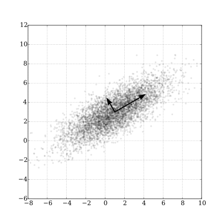
It is to maximize the variance of the data projected to some line, which means compress the information to some line as much as possible.
Let
$$Y=\arg\max{Y} var(Y)=w^{T}\Sigma w, \text{s.t.} w^T w={|w|}_2^2=1 .$$
It is an optimization problem.
| Gaussian Scatter PCA |
|---|
 |
- Principal Component Analysis Explained Visually.
- https://www.zhihu.com/question/38319536
- Principal component analysis
- https://www.wikiwand.com/en/Principal_component_analysis
- https://onlinecourses.science.psu.edu/stat505/node/49/
https://www.jianshu.com/p/d090721cf501 https://www.wikiwand.com/en/Principal_component_regression https://learnche.org/pid/latent-variable-modelling/principal-components-regression
Graph is mathematical abstract or generalization of the connection between entries.
A graph
Graphs provide a powerful way to represent and exploit these connections. Graphs can be used to model such diverse areas as computer vision, natural language processing, and recommender systems. [^12]
The connections can be directed, weighted even probabilistic.
Definition: Let
$G$ be a graph with$V(G) = {1,\dots,n}$ and$E(G) = {e_1,\dots, e_m}$ . Suppose each edge of$G$ is assigned an orientation, which is arbitrary but fixed. The (vertex-edge)incidencematrix of$G$ , denoted by$Q(G)$ , is the$n \times m$ matrix defined as follows. The rows and the columns of$Q(G)$ are indexed by$V(G)$ and$E(G)$ , respectively. The$(i, j)$ -entry of$Q(G)$ is 0 if vertex$i$ and edge$e_j$ are not incident, and otherwise it is$\color{red}{\text{1 or −1}}$ according as$e_j$ originates or terminates at$i$ , respectively. We often denote$Q(G)$ simply by$Q$ . Whenever we mention$Q(G)$ it is assumed that the edges of$G$ are oriented
Definition: Let
$G$ be a graph with$V(G) = {1,\dots,n}$ and$E(G) = {e_1,\dots, e_m}$ .Theadjacencymatrix of$G$ , denoted by$A(G)$ , is the$n\times n$ matrix defined as follows. The rows and the columns of$A(G)$ are indexed by$V(G)$ . If$i \not= j$ then the$(i, j)$ -entry of$A(G)$ is$0$ for vertices$i$ and$j$ nonadjacent, and the$(i, j)$ -entry is$\color{red}{\text{1}}$ for$i$ and$j$ adjacent. The$(i,i)$ -entry of$A(G)$ is 0 for$i = 1,\dots,n.$ We often denote$A(G)$ simply by$A$ .Adjacency Matrixis also used to representweighted graphs. If the$(i,i)$ -entry of$A(G)$ is$w_{i,j}$ , i.e.$A[i][j] = w_{i,j}$ , then there is an edge from vertex$i$ to vertex$j$ with weight$w$ . TheAdjacency Matrixofweighted graphs$G$ is also calledweightmatrix of$G$ , denoted by$W(G)$ or simply by$W$ .
See Graph representations using set and hash at https://www.geeksforgeeks.org/graph-representations-using-set-hash/.
Definition: In graph theory, the degree (or valency) of a vertex of a graph is the number of edges incident to the vertex, with loops counted twice. From the Wikipedia page at https://www.wikiwand.com/en/Degree_(graph_theory). The degree of a vertex
$v$ is denoted$\deg(v)$ or$\deg v$ .Degree matrix$D$ is a diagonal matrix such that$D_{i,i}=\sum_{j} w_{i,j}$ for theweighted graphwith$W=(w_{i,j})$ .
Definition: Let
$G$ be a graph with$V(G) = {1,\dots,n}$ and$E(G) = {e_1,\dots, e_m}$ .TheLaplacianmatrix of$G$ , denoted by$L(G)$ , is the$n\times n$ matrix defined as follows. The rows and the columns of$L(G)$ are indexed by$V(G)$ . If$i \not= j$ then the$(i, j)$ -entry of$L(G)$ is$0$ for vertices$i$ and$j$ nonadjacent, and the$(i, j)$ -entry is$\color{red}{\text{ −1}}$ for$i$ and$j$ adjacent. The$(i,i)$ -entry of$L(G)$ is$\color{red}{d_i}$ , the degree of the vertex$i$ , for$i = 1,\dots,n.$ In other words, the$(i,i)$ -entry of$L(G)$ , $L(G){i,j}$, is defined by $$L(G){i,j} = \begin{cases} \deg(V_i) & \text{if$i=j$ ,}\ -1 & \text{if$i\not= j$ and$V_i$ and$V_j$ is adjacent,} \ 0 & \text{otherwise.}\end{cases}$$ Laplacian matrix of a graph$G$ withweighted matrix$W$ is${L^{W}=D-W}$ , where$D$ is the degree matrix of$G$ . We often denote$L(G)$ simply by$L$ .
Definition: A directed graph (or
digraph) is a set of vertices and a collection of directed edges that each connects an ordered pair of vertices. We say that a directed edge points from the first vertex in the pair and points to the second vertex in the pair. We use the names 0 through V-1 for the vertices in a V-vertex graph. Via https://algs4.cs.princeton.edu/42digraph/.
It seems that graph theory is the application of matrix theory at least partially.
| Cayley graph of F2 in Wikimedia | Moreno Sociogram 1st Grade |
|---|---|
 |
 |
- http://mathworld.wolfram.com/Graph.html
- https://www.wikiwand.com/en/Graph_theory
- https://www.wikiwand.com/en/Gallery_of_named_graphs
- https://www.wikiwand.com/en/Laplacian_matrix
- http://www.ericweisstein.com/encyclopedias/books/GraphTheory.html
- https://www.wikiwand.com/en/Cayley_graph
- http://mathworld.wolfram.com/CayleyGraph.html
- https://www.wikiwand.com/en/Network_science
- https://www.wikiwand.com/en/Directed_graph
- https://www.wikiwand.com/en/Directed_acyclic_graph
- http://ww3.algorithmdesign.net/sample/ch07-weights.pdf
- https://www.geeksforgeeks.org/graph-data-structure-and-algorithms/
- https://www.geeksforgeeks.org/graph-types-and-applications/
- https://github.com/neo4j-contrib/neo4j-graph-algorithms
- https://algs4.cs.princeton.edu/40graphs/
- http://networkscience.cn/
- http://yaoyao.codes/algorithm/2018/06/11/laplacian-matrix
- The book Graphs and Matrices https://www.springer.com/us/book/9781848829800
- The book Random Graph https://www.math.cmu.edu/~af1p/BOOK.pdf.
In computer science, A* (pronounced "A star") is a computer algorithm that is widely used in pathfinding and graph traversal, which is the process of finding a path between multiple points, called "nodes". It enjoys widespread use due to its performance and accuracy. However, in practical travel-routing systems, it is generally outperformed by algorithms which can pre-process the graph to attain better performance, although other work has found A* to be superior to other approaches. It is draw from Wikipedia page on A* algorithm.
First we learn the Dijkstra's algorithm. Dijkstra's algorithm is an algorithm for finding the shortest paths between nodes in a graph, which may represent, for example, road networks. It was conceived by computer scientist Edsger W. Dijkstra in 1956 and published three years later.
| Dijkstra algorithm |
|---|
 |
- https://www.wikiwand.com/en/Dijkstra%27s_algorithm
- https://www.geeksforgeeks.org/dijkstras-shortest-path-algorithm-greedy-algo-7/
- https://www.wikiwand.com/en/Shortest_path_problem
See the page at Wikipedia A* search algorithm
Like kernels in kernel methods, graph kernel is used as functions measuring the similarity of pairs of graphs. They allow kernelized learning algorithms such as support vector machines to work directly on graphs, without having to do feature extraction to transform them to fixed-length, real-valued feature vectors.
- https://www.wikiwand.com/en/Graph_product
- https://www.wikiwand.com/en/Graph_kernel
- http://people.cs.uchicago.edu/~risi/papers/VishwanathanGraphKernelsJMLR.pdf
- https://www.cs.ucsb.edu/~xyan/tutorial/GraphKernels.pdf
- https://github.com/BorgwardtLab/graph-kernels
Spectral method is the kernel tricks applied to locality preserving projections as to reduce the dimension, which is as the data preprocessing for clustering.
In multivariate statistics and the clustering of data, spectral clustering techniques make use of the spectrum (eigenvalues) of the similarity matrix of the data to perform dimensionality reduction before clustering in fewer dimensions. The similarity matrix is provided as an input and consists of a quantitative assessment of the relative similarity of each pair of points in the data set.
Similarity matrix is to measure the similarity between the input features ${\mathbf{x}i}{i=1}^{n}\subset\mathbb{R}^{p}$. For example, we can use Gaussian kernel function $$ f(\mathbf{x_i},\mathbf{x}j)=exp(-\frac{{|\mathbf{x_i}-\mathbf{x}j|}2^2}{2\sigma^2}) $$ to measure the similarity of inputs. The element of similarity matrix $S$ is $S{i,j}=exp(-\frac{{|\mathbf{x_i}-\mathbf{x}j|}2^2}{2\sigma^2})$. Thus $S$ is symmetrical, i.e. $S{i,j}=S{j,i}$ for $i,j\in{1,2,\dots,n}$. If the sample size $n\gg p$, the storage of similarity matrix is much larger than the original input ${\mathbf{x}i}{i=1}^{n}$, when we would only preserve the entries above some values. The Laplacian matrix is defined by $L=D-S$ where $D=Diag{D_1,D_2,\dots,D_n}$ and $D{i}=\sum{j=1}^{n}S_{i,j}=\sum_{j=1}^{n}exp(-\frac{{|\mathbf{x_i}-\mathbf{x}_j|}_2^2}{2\sigma^2})$.
Then we can apply principal component analysis to the Laplacian matrix
- https://zhuanlan.zhihu.com/p/34848710
- On Spectral Clustering: Analysis and an algorithm at http://papers.nips.cc/paper/2092-on-spectral-clustering-analysis-and-an-algorithm.pdf
- A Tutorial on Spectral Clustering at https://www.cs.cmu.edu/~aarti/Class/10701/readings/Luxburg06_TR.pdf.
- 谱聚类 https://www.cnblogs.com/pinard/p/6221564.html.
- Spectral Clustering http://www.datasciencelab.cn/clustering/spectral.
- https://en.wikipedia.org/wiki/Category:Graph_algorithms
- The course Spectral Graph Theory, Fall 2015 athttp://www.cs.yale.edu/homes/spielman/561/.