The ReLU activation funtion is a nonlinear function defined as
$$\operatorname{ReLU}(x)=\sigma(x)=\max(x,0)=[x]{+}=\arg\max{x}|x-z|2^2+\chi{z>0}(z)$$
where
This operator is a projection operator so that
And we can find that
- https://www.gabormelli.com/RKB/Rectified_Linear_Unit_(ReLU)_Activation_Function
- https://sefiks.com/2017/08/21/relu-as-neural-networks-activation-function/
- https://mlfromscratch.com/activation-functions-explained/
- http://web.stanford.edu/~jlmcc/papers/PDP/Volume%201/Chap10_PDP86.pdf
- Rectified Linear Units Improve Restricted Boltzmann Machines
- http://www.cs.toronto.edu/~fritz/absps/imagenet.pdf
Here we would introduce some application of ReLU before deep learning.
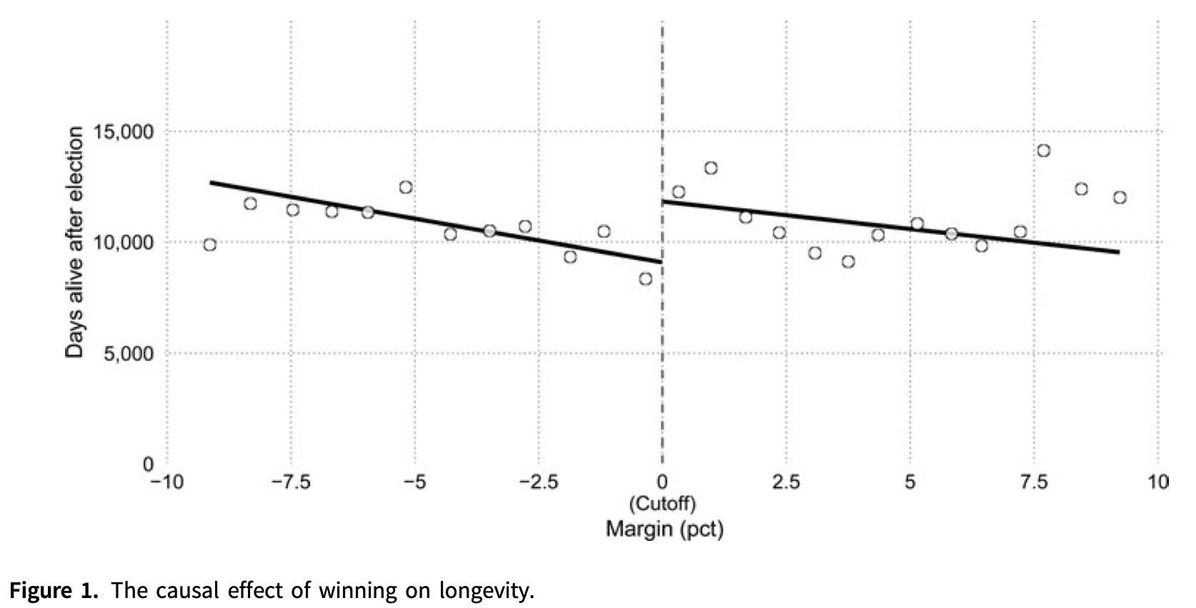
Regression discontinuity has emerged as one of the most credible
non-experimental strategies for the analysis of causal effects.
In the RD design, all units have a score, and a treatment is assigned to those units whose value of the score exceeds a known cutoff or threshold,
and not assigned to those units whose value of the score is below the cutoff.
The key feature of the design is that the probability of receiving the treatment changes abruptly at the known threshold.
If units are unable to perfectly “sort” around this threshold, the discontinuous change
in this probability can be used to learn about the local causal effect of the treatment on an outcome of interest,
because units with scores barely below the cutoff can be used as a comparison group for units with scores barely above it.
- https://statmodeling.stat.columbia.edu/2020/07/02/no-i-dont-believe-that-claim-based-on-regression-discontinuity-analysis-that/
- https://erikgahner.dk/2020/a-response-to-andrew-gelman/
- https://cattaneo.princeton.edu/books/Cattaneo-Idrobo-Titiunik_2019_CUP-Vol1.pdf
- https://cran.r-project.org/web/packages/lm.br/vignettes/lm.br.pdf
- https://www.mdrc.org/sites/default/files/RDD%20Guide_Full%20rev%202016_0.pdf
- https://pdfs.semanticscholar.org/0ebb/29615b1569e9ee219f536c9ad64ae5fce36d.pdf
- https://www.tandfonline.com/doi/abs/10.1080/19345747.2011.578707
- https://www.waterlog.info/segreg.htm
- Matching, Regression Discontinuity, Difference in Differences
- Dummy-Variable Regression
Multivariate Adaptive Regression Splines (MARS) is a method for flexible modelling of high dimensional data.
The model takes the form of an expansion in product spline basis functions,
where the number of basis functions as well as the parameters associated with each one (product degree and knot locations) are automatically determined by the data.
This procedure is motivated by recursive partitioning (e.g. CART) and shares its ability to capture high order interactions.
However, it has more power and flexibility to model relationships that are nearly additive or involve interactions in at most a few variables, and produces continuous models with continuous derivatives.
In addition, the model can be represented in a form that separately identifies the additive contributions and those associated with different multivariable interactions.
- https://publichealth.yale.edu/c2s2/software/masal/
- https://pubmed.ncbi.nlm.nih.gov/8548103/
- http://www.stat.yale.edu/~arb4/publications_files/DiscussionMultivariateAdaptiveRegressionSplines.pdf
- https://projecteuclid.org/euclid.aos/1176347963
Those pieces come together into a learning function
| Order | Component | Meaning |
|---|---|---|
| 1 | Key operation | Composition |
| 2 | Key rule | Chain rule for |
| 3 | Key algorithm | Stochastic gradient descent to find the best weights |
| 4 | Key subroutine | Backpropagation to execute the chain rule |
| 5 | Key nonlinearity |
The ReLU networks take the ReLU layers as its components:
- (1) When
$x\in\mathbb{R}$ , it is simple:$W_i\in\mathbb{R}$ . - (2) When
$x\in\mathbb{R}^n\quad \forall n\geq 2$ ,$W_i\in\mathbb{R}^{m\times n}$ so$W_ih_i$ is matrix-vector multiplication. It is a piecewise linear function no matter how large the layer number$L$ is. And$\sigma(W_Lh_L)=W_{x}x$ where$W_{x}$ is a matrix determined by the raw input$h_0(x)$ . - (3) When
$x\in\mathbb{R}^{m\times n}\quad \forall n\geq,m\geq 2$ such as in ConvNet,$W_ih_i$ is the result of the convolution operator and$W_i$ is the convolution kernel (filter).
- https://wwwhome.ewi.utwente.nl/~schmidtaj/
- https://smartech.gatech.edu/handle/1853/60957
- Nonparametric regression using deep neural networks with ReLU activation function
- Some statistical theory for deep neural networks
- Statistical guarantees for deep ReLU networks
- A Geometric Interpretation of Neural Networks
- A comparison of deep networks with ReLU activation function and linear spline-type methods
ReLU Networks Approximation and Expression Ability
We can use the ReLU function to approximate an indictor function:
$$\sigma(x)-\sigma(x-\frac{1}{a})=\begin{cases}
0, &\text{if
- Optimal Approximation with Sparse Deep Neural Networks
- Provable approximation properties for deep neural networks
- http://www.spartan-itn.eu/#0
- Shearlets: Multiscale Analysis for Multivariate Data
And we can use it to generate more functions such as
- Every continuous function can be approximated up to an
error of
$\varepsilon > 0$ with a neural network with a single hidden layer and with$O(N)$ neurons. - We can leads to appropriate shearlet generator with neural networks.
- Deep neural networks are optimal for the approximation of piecewise smooth functions on manifolds.
- For certain topologies, the standard backpropagation algorithm generates a deep neural network which provides those optimal approximation rates; interestingly even yielding
$\alpha$ -shearlet-like functions.
- http://www.math.tu-berlin.de/%E2%88%BCkutyniok
- Nonlinear Approximation and (Deep) ReLU Networks
- https://www2.isye.gatech.edu/~tzhao80/
- New Error Bounds for Deep ReLU Networks Using Sparse Grids
- Deep ReLU network approximation of functions on a manifold
- Explaining Nonparametric Regression on Low Dimensional Manifolds using Deep Neural Networks
- Universal Function Approximation by Deep Neural Nets with Bounded Width and ReLU Activations
- https://www.stat.uchicago.edu/~lekheng/work/reprints.html
- A Note On The Expressive Power Of Deep ReLU Networks In High-Dimensional Space
- How degenerate is the parametrization of neural networks with the ReLU activation function?
- On the Expressive Power of Deep Neural Networks
- Optimal approximation of piecewise smooth functions using deep ReLU neural networks
- Optimal approximation of continuous functions by very deep ReLU networks
- https://www.mins.ee.ethz.ch/people/show/boelcskei
- https://mat.univie.ac.at/~grohs/
Here we show that a deep convolutional neural network (CNN) is universal, meaning that it can be used to approximate any continuous function to an arbitrary accuracy when the depth of the neural network is large enough. This answers an open question in learning theory. Our quantitative estimate, given tightly in terms of the number of free parameters to be computed, verifies the efficiency of deep CNNs in dealing with large dimensional data. Our study also demonstrates the role of convolutions in deep CNNs.
- https://www.cityu.edu.hk/rcms/DXZhou.htm
- Universality of deep convolutional neural networks
- Deep Distributed Convolutional Neural Networks: Universality
- Deep Learning using Rectified Linear Units (ReLU)
- Deep Sparse Rectifier Neural Networks
- Provable Robustness of ReLU networks via Maximization of Linear Regions
- https://deepai.org/publication/dying-relu-and-initialization-theory-and-numerical-examples
- http://www.columbia.edu/cu/neurotheory/Larry/SalinasPNAS96.pdf
- http://www.cs.toronto.edu/~ranzato/publications/zeiler_icassp13.pdf
- https://www.math.tamu.edu/~bhanin/
- https://link.springer.com/article/10.1007%2Fs10462-019-09752-1
- https://www.microsoft.com/en-us/research/people/wche/publications/
- https://www.math.uci.edu/~jxin/RVSCGD_2020.pdf
- https://chulheey.mit.edu/
- http://aisociety.kr/KJMLW2019/slides/suzuki.pdf
- https://deepai.org/publication/ginn-geometric-illustration-of-neural-networks
- Reverse-Engineering Deep ReLU Networks
- https://www.stat.uchicago.edu/~lekheng/work/tropical.pdf
- https://deepai.org/profile/jeffrey-pennington
- https://deepai.org/publication/the-emergence-of-spectral-universality-in-deep-networks
- https://github.com/fwcore/mean-field-theory-deep-learning
- https://www.zhihu.com/question/360303367
- https://www.bayeswatch.com/2018/09/17/GINN/
Convergence
- https://github.com/facebookresearch/luckmatters
- Luck Matters: Understanding Training Dynamics of Deep ReLU Networks
- G-SGD: Optimizing ReLU Neural Networks in its Positively Scale-Invariant Space
- A Convergence Theory for Deep Learning via Over-Parameterization
- https://arxiv.org/abs/1703.00560
- http://www.yuandong-tian.com/Yuandong_TheoreticalFramework_48x36.pdf
- https://arxiv.org/abs/1809.10829
- https://arxiv.org/abs/1705.09886
- https://arxiv.org/abs/2002.04763
- https://arxiv.org/abs/1909.13458
- https://arxiv.org/pdf/1903.12384.pdf
- http://www.yuandong-tian.com/
- http://people.csail.mit.edu/shubhendu/
- https://openreview.net/pdf?id=Hk85q85ee
- https://ieeexplore.ieee.org/document/8671751
- https://arxiv.org/pdf/1906.00904.pdf
Generalization of Deep ReLU Networks
Recently, path norm was proposed as a new capacity measure for neural networks with Rectified Linear Unit (ReLU) activation function, which takes the rescaling-invariant property of ReLU into account. It has been shown that the generalization error bound in terms of the path norm explains the empirical generalization behaviors of the ReLU neural networks better than that of other capacity measures. Moreover, optimization algorithms which take path norm as the regularization term to the loss function, like Path-SGD, have been shown to achieve better generalization performance. However, the path norm counts the values of all paths, and hence the capacity measure based on path norm could be improperly influenced by the dependency among different paths. It is also known that each path of a ReLU network can be represented by a small group of linearly independent basis paths with multiplication and division operation, which indicates that the generalization behavior of the network only depends on only a few basis paths. Motivated by this, we propose a new norm Basis-path Norm based on a group of linearly independent paths to measure the capacity of neural networks more accurately. We establish a generalization error bound based on this basis path norm, and show it explains the generalization behaviors of ReLU networks more accurately than previous capacity measures via extensive experiments. In addition, we develop optimization algorithms which minimize the empirical risk regularized by the basis-path norm. Our experiments on benchmark datasets demonstrate that the proposed regularization method achieves clearly better performance on the test set than the previous regularization approaches.
- https://dblp.uni-trier.de/pers/z/Zhang:Chiyuan.html
- Deep learning and structured data
- https://www.paperswithcode.com/paper/why-relu-networks-yield-high-confidence
- https://arxiv.org/pdf/1910.08581.pdf
- https://intra.ece.ucr.edu/~oymak/asilomar19.pdf
- https://arxiv.org/pdf/1911.12360.pdf
- https://www.dtc.umn.edu/s/resources/spincom8526.pdf
Finite Element