Statistical Foundations of Data Science by Jianqing Fan, Runze Li, Cun-Hui Zhang, Hui Zhou discussed advanced latest topics in high dimensional statistics. High-Dimensional Probability: An Introduction with Applications in Data Science is a company to the previous one.
The curse of high dimensionality and the bless of high dimensionality is the core topic of the high dimensional statistics in my belief.
New and Evolving Roles of Shrinkage in Large-Scale Prediction and Inference (19w5188)
Regression is a method for studying the relationship between a response variable
Regression is not function fitting. In function fitting, it is well-defined -
Linear regression is the "hello world" in statistical learning. It is the simplest model to fit the datum. We will induce it in the maximum likelihood estimation perspective. See this link for more information https://www.wikiwand.com/en/Regression_analysis.
A linear regression model assumes that the regression function
By convention (very important!):
-
$\mathrm{x}$ is assumed to be standardized (mean 0, unit variance); -
$\mathrm{y}$ is assumed to be centered.
For the linear regression, we could assume
The likelihood of the errors are
$$
L(\epsilon_1,\epsilon_2,\cdots,\epsilon_n)=\prod_{i=1}^{n}\frac{1}{\sqrt{2\pi}}e^{-\epsilon_i^2}.
$$
In MLE, we have shown that it is equivalent to $$ \arg\max \prod_{i=1}^{n}\frac{1}{\sqrt{2\pi}}e^{-\epsilon_i^2}=\arg\min\sum_{i=1}^{n}\epsilon_i^2=\arg\min\sum_{i=1}^{n}(y_i-f(x_i))^2. $$
| Linear Regression and Likelihood Maximum Estimation |
|---|
 |
For linear regression, the function
where
- the residual error
${\epsilon_i}_{i=1}^{n}$ are i.i.d. in Gaussian distribution; - the inverse matrix
$(X^{T}X)^{-1}$ may not exist in some extreme case.
See more on Wikipedia page.
When the matrix
In the perspective of computation, we would like to consider the regularization technique; In the perspective of Bayesian statistics, we would like to consider more proper prior distribution of the parameters.
It is to optimize the following objective function with parameter norm penalty
$$
PRSS_{\ell_2}=\sum_{i=1}^{n}(y_i-w^Tx_i)^2+\lambda w^{T}w=|Y-Xw|^2+\lambda|w|^2,\tag {Ridge}.
$$
It is called penalized residual sum of squares.
Taking derivatives, we solve
$$
\frac{\partial PRSS_{\ell_2}}{\partial w}=2X^T(Y-Xw)+2\lambda w=0
$$
and we gain that
$$
w=(X^{T}X+\lambda I)^{-1}X^{T}Y
$$
where it is trackable if
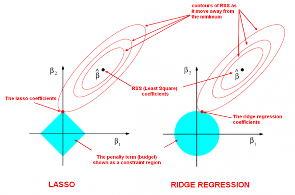
LASSO is the abbreviation of Least Absolute Shrinkage and Selection Operator.
-
It is to minimize the following objective function: $$ PRSS_{\ell_1}=\sum_{i=1}^{n}(y_i-w^Tx_i)^2+\lambda{|w|}_{1} =|Y-Xw|^2+\lambda{|w|}_1,\tag {LASSO}. $$
-
the optimization form: $$ \arg\min_{w}\sum_{i=1}^{n}(y_i-w^Tx_i)^2 \qquad\text{objective function} \ \text{subject to},{|w|}_1 \leq t \qquad\text{constraint}. $$
-
the selection form: $$ \arg\min_{w}{|w|}1 \qquad \text{objective function} \ \text{subject to},\sum{i=1}^{n}(y_i-w^Tx_i)^2 \leq t \qquad \text{constraint}. $$ where ${|w|}1=\sum{i=1}^{n}|w_i|$ if
$w=(w_1,w_2,\cdots, w_n)^{T}$ .
| LASSO and Ridge Regression |
|---|
 |
| The LASSO Page ,Wikipedia page and Q&A in zhihu.com |
| More References in Chinese blog |
If we suppose the prior distribution of the parameters
Iterative Shrinkage-Threshold Algorithms(ISTA) for
FISTA with constant stepsize
$x^{k}= p_{L}(y^k)$ computed as ISTA;$t_{k+1}=\frac{1+\sqrt{1+4t_k^2}}{2}$ ;$y^{k+1}=x^k+\frac{t_k -1}{t_{k+1}}(x^k-x^{k-1})$ .
- A Fast Iterative Shrinkage Algorithm for Convex Regularized Linear Inverse Problems
- https://pylops.readthedocs.io/en/latest/gallery/plot_ista.html
- ORF523: ISTA and FISTA
- Fast proximal gradient methods, EE236C (Spring 2013-14)
- https://github.com/tiepvupsu/FISTA
- A Fast Iterative Shrinkage-Thresholding Algorithm for Linear Inverse Problems
- ADMM Algorithmic Regularization Paths for Sparse Statistical Machine Learning
More solutions to this optimization problem:
- http://www.cnblogs.com/xingshansi/p/6890048.html
- Q&A in zhihu.com;
- LASSO using ADMM;
- Regularization: Ridge Regression and the LASSO;
- Least angle regression;
- http://web.stanford.edu/~hastie/StatLearnSparsity/
- 历史的角度来看,Robert Tibshirani 的 Lasso 到底是不是革命性的创新?- 若羽的回答 - 知乎
- An Homotopy Algorithm for the Lasso with Online Observations
- The Solution Path of the Generalized Lasso
Generally, we may consider the penalty residual squared sum $$ PRSS_{\ell_p}=\sum_{i=1}^{n}(y_i -w^T x_i)^2+\lambda{|w|}{p}^{p} =|Y -X w|^2+\lambda{|w|}p^{p},\tag {LASSO} $$ where ${|w|}{p}=(\sum{i=1}^{n}|w_i|^{p})^{1/p}, p\in (0,1)$.
Dr. Zongben Xu proposed the
When the sample size of training data
See more on http://web.stanford.edu/~hastie/TALKS/glmnet_webinar.pdf or http://www.princeton.edu/~yc5/ele538_math_data/lectures/model_selection.pdf.
We can deduce it by Bayesian estimation if we suppose the prior distribution of the parameters
See Bayesian lasso regression at http://faculty.chicagobooth.edu/workshops/econometrics/past/pdf/asp047v1.pdf.
The nonconvex approach leads to the following optimization problem: $$ \min_{x\in\mathbb{R}^{p}} J(x) = \frac{1}{2}{|Ax-b|}2^2+\sum{i=1}^{p}{\rho}_{\lambda,\tau}(x_i) $$
where ${\rho}{\lambda,\tau}$ is nonconvex penalty, $\lambda>0$ is a regularization parameter and $\tau$ controls the degree of convexity of the penalty. Because the cost function is separable, we will define a thresholding operator $S^{\rho}{\lambda, \tau}$ with respect of the penalty ${\rho}{\lambda,\tau}$: $$S^{\rho}{\lambda, \tau}(v)=\arg\min_{u\in\mathbb{R}^p}{\frac{(u-v)^2}{2}+{\rho}_{\lambda,\tau}(u)}$$
- LASSO: ${\rho}{\lambda,\tau}=\lambda |t|$, $S{\lambda,\tau}^{\rho}(v) = sgn(v){(|v| -\lambda)}_{+}$;
- SCAD,
$\tau>2$ , $$ {\rho}_{\lambda,\tau}(t) = \begin{cases} \lambda |t|, &\text{$|t|\leq\lambda$}\ \frac{\lambda\tau|t|-\frac{1}{2}(t^2+\lambda^2)}{2}, &\text{$\lambda<|t|\leq\lambda\tau$}\ \frac{\lambda^2(\tau +1)}{2}, &\text{$|t|>\lambda\tau$} \end{cases}. $$
- MCP,
$\tau >1$ , $$ {\rho}_{\lambda,\tau}(t) = \begin{cases} \lambda (|t|-\frac{t^2}{2\lambda \tau}), &\text{if$|t|<\tau\lambda$ } \ \frac{\lambda^2\tau}{2}, &\text{if$|t|\geq \tau\lambda$ } \end{cases}. $$
- http://dsp.rice.edu/cs/
- A Unifi ed Primal Dual Active Set Algorithm for Nonconvex Sparse Recovery
- Sparsity and Compressed Sensing
- Compressed Sensing at cnx.org
- ELE538B: Sparsity, Structure and Inference, Yuxin Chen, Princeton University, Spring 2017
- Stats 330 (CME 362) An Introduction to Compressed Sensing Spring 2010
- Statistical Learning with Sparsity: The Lasso and Generalizations
In this chapter we discuss prediction problems in which the number of
features
The outcome
where
Suppose
- http://www.biostat.jhsph.edu/~iruczins/teaching/jf/ch10.pdf
- https://newonlinecourses.science.psu.edu/stat508/
- High-dimensional variable selection
- Nearly unbiased variable selection under minimax concave penalty
- Coordinate descent algorithms for nonconvex penalized regression, with applications to biological feature selection
- The composite absolute penalties family for grouped and hierarchical variable selection
- MAP model selection in Gaussian regression
- “Preconditioning” for feature selection and regression in high-dimensional problems
- A Selective Overview of Variable Selection in High Dimensional Feature Space
- Variable selection – A review and recommendations for the practicing statistician
- Comparison of the modified unbounded penalty and the LASSO to select predictive genes of response to chemotherapy in breast cancer
- Variable Selection via Nonconcave Penalized Likelihood and its Oracle Properties, Jianqing Fan and Li R. JASO