In ordinary least squares, we assume that the errors ({ { \epsilon }{i} }{i=1}^{n}) are i.i.d. Gaussian, i.e.
Ordinary linear regression predicts the expected value of a given unknown quantity (the response variable, a random variable) as a linear combination of a set of observed values (predictors). This implies that a constant change in a predictor leads to a constant change in the response variable (i.e. a linear-response model). This is appropriate when the response variable has a normal distribution (intuitively, when a response variable can vary essentially indefinitely in either direction with no fixed "zero value", or more generally for any quantity that only varies by a relatively small amount, e.g. human heights).
However, these assumptions are inappropriate for some types of response variables. For example, in cases where the response variable is expected to be always positive and varying over a wide range, constant input changes lead to geometrically varying, rather than constantly varying, output changes. As an example, a prediction model might predict that 10 degree temperature decrease would lead to 1,000 fewer people visiting the beach is unlikely to generalize well over both small beaches (e.g. those where the expected attendance was 50 at a particular temperature) and large beaches (e.g. those where the expected attendance was 10,000 at a low temperature). The problem with this kind of prediction model would imply a temperature drop of 10 degrees would lead to 1,000 fewer people visiting the beach, a beach whose expected attendance was 50 at a higher temperature would now be predicted to have the impossible attendance value of −950. Logically, a more realistic model would instead predict a constant rate of increased beach attendance (e.g. an increase in 10 degrees leads to a doubling in beach attendance, and a drop in 10 degrees leads to a halving in attendance). Such a model is termed an exponential-response model (or log-linear model, since the logarithm of the response is predicted to vary linearly).
In a generalized linear model (GLM), each outcome
The GLM consists of three elements:
| Model components |
|---|
| 1. A probability distribution from the exponential family. |
| 2. A linear predictor |
| 3. A link function |
- https://xg1990.com/blog/archives/304
- https://zhuanlan.zhihu.com/p/22876460
- https://www.wikiwand.com/en/Generalized_linear_model
- Roadmap to generalized linear models in metacademy at (https://metacademy.org/graphs/concepts/generalized_linear_models#lfocus=generalized_linear_models)
- Course in Princeton
- Exponential distribution familiy
- 14.1 - The General Linear Mixed Model
- https://scikit-learn.org/stable/modules/linear_model.html#
- Multilevel model https://www.wikiwand.com/en/Multilevel_model
- Hierarchical generalized linear model https://www.wikiwand.com/en/Hierarchical_generalized_linear_model
- http://bactra.org/notebooks/regression.html
An exponential family distribution has the following form $$ p(x|\eta)=h(x) \exp(\eta^{T}t(x) - a(\eta)) $$ where
- a parameter vector
$\eta$ is often referred to as the canonical or natural parameter; - the statistic
$t(X)$ is referred to as asufficient statistic; - the underlying measure
$h(x)$ is a counting measure or Lebesgue measure; - the log normalizer
$a(\eta)=\log \int h(x) \exp(\eta^{T}t(x)) \mathrm{d}x$
For example, a Bernoulli random variable
$$
p(x|\eta)
= {\pi}^{x}(1-\pi)^{1-x}\
= {\frac{\pi}{1-\pi}}^{x} (1-\pi)\
= \exp{\log(\frac{\pi}{1-\pi})x+\log (1-\pi)}
$$
so that
The Poisson distribution can be written in
$$
p(x|\lambda)
=\frac{{\lambda}^{x}e^{-\lambda}}{x!} \
= \frac{1}{x!}exp{x\log(\lambda)-\lambda}
$$
for
| --- | --- |
|---|---|
|
|
The multinomial distribution can be written in $$ p(x|\pi) =\frac{M!}{{x}{1}!{x}{2}!\cdots {x}{K}!}{\pi}{1}^{x_1}{\pi}{2}^{x_2}\cdots {\pi}{K}^{x_K} \ = \frac{M!}{{x}{1}!{x}{2}!\cdots {x}{K}!}\exp{\sum{i=1}^{K}x_i\log(\pi_i)} \ = \frac{M!}{{x}{1}!{x}{2}!\cdots {x}{K}!}\exp{\sum{i=1}^{K-1}x_i\log(\pi_i)+(M-\sum_{i=1}^{K-1}x_i) \log(1-\sum_{i=1}^{K-1} \pi_i)} \ = \frac{M!}{{x}{1}!{x}{2}!\cdots {x}{K}!}\exp{\sum{i=1}^{K-1}x_i\log(\frac{\pi_i}{1-\sum_{i=1}^{K-1} \pi_i}) + M \log(1-\sum_{i=1}^{K-1} \pi_i)} $$
where
-
$\eta_k =\log(\frac{\pi_k}{1-\sum_{i=1}^{K-1} \pi_i})=\log(\frac{\pi_k}{\pi_K})$ then$\pi_k = \frac{e^{\eta_k}}{\sum_{k=1}^{K}e^{\eta_k}}$ for$k\in{1,2,\dots, K}$ with$\eta_K = 0$ ; -
$t(X)=X=(X_1, X_2, \dots, X_{K-1})$ ; - $h(x)=\frac{M!}{{x}{1}!{x}{2}!\cdots {x}_{K}!}$;
-
$a(\eta)=-M \log(1-\sum_{i=1}^{K-1} \pi_i)=-M \log(\pi_K)$ .
Note that
- https://en.wikipedia.org/wiki/Exponential_family
- https://www.cs.princeton.edu/courses/archive/fall11/cos597C/lectures/exponential-families.pdf
- https://people.eecs.berkeley.edu/~jordan/courses/260-spring10/other-readings/chapter8.pdf
| Logistic Regression |
|---|
| 1. A Bernoulli random variable |
| 2. A linear predictor |
| 3. A link function |
The logistic distribution: $$ \pi\stackrel{\triangle}=P(Y=1|X=x)=\frac{1}{1+e^{-x^{T}\beta}}=\frac{e^{x^{T}\beta}}{1+e^{x^{T}\beta}} $$
where
i.e. logistic (or logit) transformation,
where
How we can do estimate the parameters
The log-likelihood turns products into sums $$ \ell(\beta) ={\sum}{i=1}^{n}{y}{i}\log(\pi)+(1-{y}i)\log(1-\pi) \ = {\sum}{i=1}^{n}{y}{i}\log(\frac{\pi}{1-\pi})+\log(1-\pi) \ = {\sum}{i=1}^{n}{y}_{i}(x_i^T\beta)-\log(1+\exp(x_i^T\beta)) $$
where
$$ \hat{\beta} = \arg\max_{\beta} L(\beta)=\arg\max_{\beta} \ell(\beta) \ = \arg\max_{\beta} {\sum}{i=1}^{n}{y}{i}(x_i^T\beta)-\log(1+\exp(x_i^T\beta)) $$
which we can solve this optimization by numerical optimization methods such as Newton's method.
$$\arg\max_{\beta} L(\beta)={\sum}{i=1}^{n}{y}{i}\log(\pi)+(1-{y}_i)\log(1-\pi) $$
- https://www.wikiwand.com/en/Logistic_regression
- https://www.stat.cmu.edu/~cshalizi/uADA/12/lectures/ch12.pdf
- https://machinelearningmastery.com/logistic-regression-for-machine-learning/
- http://www.omidrouhani.com/research/logisticregression/html/logisticregression.htm
- How is Ethics Like Logistic Regression?
- TOP SECRET: Newly declassified documents on evaluating models based on predictive accuracy
- 逻辑回归(logistic regression)的本质——极大似然估计
Poisson regression assumes the response variable
| Poisson Regression |
|---|
| 1. A Poisson random variable |
| 2. A linear predictor |
| 3. A link function |
Thus we obtain that
$$ \ell(\beta|X, Y) = {\sum}{i=1}^{n}[y_i x_i^T\beta -\exp(x_i^T\beta)-\log(y_i!)] \ \propto {\sum}{i=1}^{n} [y_i x_i^T\beta -\exp(x_i^T\beta)]. $$
The negative log-likelihood function
| Softmax Regression |
|---|
| 1. A multinomial random variable |
| 2. A linear predictor |
| 3. A link function |
The log-likelihood in terms of
- http://ufldl.stanford.edu/wiki/index.php/Softmax%E5%9B%9E%E5%BD%92
- https://www.wikiwand.com/en/Multinomial_logistic_regression
- https://www.wikiwand.com/en/Softmax_function
- https://metacademy.org/graphs/concepts/multinomial_logistic_regression
Generalized linear models extend the distribution of outputs so that the loss function(the likelihood function or log-likelihood function).
It is supposed that there is a link function
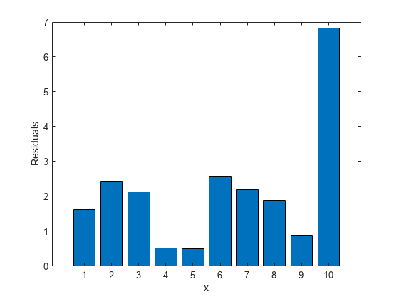
Robust regression can be used in any situation in which you would use least squares regression. When fitting a least squares regression, we might find some outliers or high leverage data points. We have decided that these data points are not data entry errors, neither they are from a different population than most of our data. So we have no compelling reason to exclude them from the analysis. Robust regression might be a good strategy since it is a compromise between excluding these points entirely from the analysis and including all the data points and treating all them equally in OLS regression. The idea of robust regression is to weigh the observations differently based on how well behaved these observations are. Roughly speaking, it is a form of weighted and reweighted least squares regression. Draw form[https://stats.idre.ucla.edu/r/dae/robust-regression/].
For our first robust regression method, suppose we have a data set of size n such that
where
M-estimators are given by
$$
\hat{\beta}M=\arg\min{\beta}{\sum}_{i}\rho({\epsilon}_i)
$$
where
The M stands for "maximum likelihood" since
- Nonnegative,
$\rho(e)\geq 0 ,,\forall e$ ; - Equal to zero when its argument is zero,
$\rho(0)=0$ ; - Symmetric,
$\rho(e)=\rho(-e)$ ; - Monotone in
$|e|$ ,$\rho(e_1)\geq \rho(e_2)$ if$|e_1|>|e_2|$ .
For example,
|Method|Loss function| |:---|:---:|---:| |Least-Squares|$\rho_{LS}(e)=e^2$| |Huber | Huber function |Bisquare|mathworld| |Winsorizing|Wiki page|

Three common functions chosen in M-estimation are given in Robust Regression Methods.
And it is really close to supervised machine learning.
- https://stats.idre.ucla.edu/r/dae/robust-regression/
- http://users.stat.umn.edu/~sandy/courses/8053/handouts/robust.pdf
- https://newonlinecourses.science.psu.edu/stat501/node/351/
- https://stats.idre.ucla.edu/r/dae/robust-regression/
- https://www.r-bloggers.com/visual-contrast-of-two-robust-regression-methods/
- https://newonlinecourses.science.psu.edu/stat501/node/353/
- https://projecteuclid.org/euclid.aos/1534492823
- https://orfe.princeton.edu/~jqfan/papers/14/Robust14.pdf
Another application of design loss function is in feature selection or regularization such as LASSO, SCAD.
Given samples spline with knots at some prespecified locations
The regularization technique can be applied to control the model complexity
It can date back to spline interpolation in computational or numerical analysis. There may be some points such as ploynomial regression:
- http://www.stat.cmu.edu/~ryantibs/advmethods/notes/smoothspline.pdf
- https://web.stanford.edu/class/stats202/content/lec17.pdf
- https://robjhyndman.com/etc5410/splines.pdf
- https://newonlinecourses.science.psu.edu/stat501/node/324/
In the regression setting, a generalized additive model has the form
There is a section of projection pursuit and neural networks in Element of Statistical Learning.
Assume we have an input vector
where each parameter projection indices.
The function
The single index model in econometrics.
We seek the approximate minimizers of the error function $$ \sum_{n=1}^{N}[y_n - \sum_{m=1}^{M} g_m ( \left<\omega_m, x_i \right>)]^2 $$
over functions
And there is a PHD thesis Design and choice of projection indices in 1992.
- https://www.wikiwand.com/en/Projection_pursuit_regression
- https://projecteuclid.org/euclid.aos/1176349519
- https://projecteuclid.org/euclid.aos/1176349520
- https://projecteuclid.org/euclid.aos/1176349535
- https://people.maths.bris.ac.uk/~magpn/Research/PP/PP.html
- https://www.wikiwand.com/en/Projection_pursuit_regression
- http://www.stat.cmu.edu/~larry/=stat401/
- http://cis.legacy.ics.tkk.fi/aapo/papers/IJCNN99_tutorialweb/node23.html
- https://www.pnas.org/content/115/37/9151
- https://www.ncbi.nlm.nih.gov/pubmed/30150379
In generalized linear model, the response
The assumption for the straight-line model is:
-
Our straight-line model is $$ Y_i = \alpha + \beta x_i + e_i, i=1,2,\dots, n $$ where distinct
$x_i$ is known observed constants and$\alpha$ and$\beta$ are unknown parameters to estimate. -
The random variables
$e_i$ are random sample from a continuous population that has median 0.
Then we would make a null hypothesis
and Theil construct a statistics
where
For different alternative hypothesis, we can test it via comparing with the p-values.
- https://jvns.ca/blog/2018/12/29/some-initial-nonparametric-statistics-notes/
- https://www.wikiwand.com/en/Additive_model
- https://www.wikiwand.com/en/Generalized_additive_model
- http://iacs-courses.seas.harvard.edu/courses/am207/blog/lecture-20.html
- Nonparametric regression https://www.wikiwand.com/en/Nonparametric_regression
- http://www.stat.cmu.edu/~larry/=sml
- http://www.stat.cmu.edu/~larry/
- https://zhuanlan.zhihu.com/p/26830453
- http://wwwf.imperial.ac.uk/~bm508/teaching/AppStats/Lecture7.pdf
- http://web.stanford.edu/class/ee378a/books/book2.pdf
Bayesian nonparametric (BNP) approach is to fit a single model that can adapt its complexity to the data. Furthermore, BNP models allow the complexity to grow as more data are observed, such as when using a model to perform prediction.
Please remind the Bayesian formula: $$ P(A|B)=\frac{P(B|A)P(A)}{P(B)}\ P(A|B)\propto P(B|A)P(A) $$
and in Bayesian everything can be measured in the belief degree in
Each model expresses a generative process of the data that includes hidden variables. This process articulates the statistical assumptions that the model makes, and also specifies the joint probability distribution of the hidden and observed random variables. Given an observed data set, data analysis is performed by posterior inference, computing the conditional distribution of the hidden variables given the observed data.
- A Tutorial on Bayesian Nonparametric Models
- https://www.quantstart.com/articles/Bayesian-Linear-Regression-Models-with-PyMC3
- http://doingbayesiandataanalysis.blogspot.com/2012/11/shrinkage-in-multi-level-hierarchical.html
- https://twiecki.github.io/blog/2013/08/12/bayesian-glms-1/
- https://twiecki.github.io/blog/2013/08/27/bayesian-glms-2/
- https://twiecki.github.io/blog/2014/03/17/bayesian-glms-3/
- https://blog.applied.ai/bayesian-inference-with-pymc3-part-1/
- https://blog.applied.ai/bayesian-inference-with-pymc3-part-2/
- https://blog.applied.ai/bayesian-inference-with-pymc3-part-3/
- https://magesblog.com/post/2016-02-02-first-bayesian-mixer-meeting-in-london/
- https://www.meetup.com/Bayesian-Mixer-London/
- https://sites.google.com/site/doingbayesiandataanalysis/