The simple function is a real-valued function
The tree-based learning algorithms take advantages of these universal approximators to fit the decision function.

The core problem is to find the optimal parameters
In brief, A decision tree is a classifier expressed as a recursive partition of the instance space.
A decision tree is the function
$T :\mathbb{R}^d \to \mathbb{R}$ resulting from a learning algorithm applied on training data lying in input space$\mathbb{R}^d$ , which always has the following form: $$ T(x) = \sum_{i\in\text{leaves}} g_i(x)\mathbb{I}(x\in R_i) = \sum_{i\in ,\text{leaves}} g_i(x) \prod_{a\in,\text{ancestors(i)}} \mathbb{I}(S_{a (x)}=c_{a,i}) $$ where$R_i \subset \mathbb{R}^d$ is the region associated with leaf${i}$ of the tree,$\text{ancestors(i)}$ is the set of ancestors of leaf node i,$c_{a,i}$ is the child of node a on the path from a to leaf i, and$S_a$ is the n-array split function at node a.$g_i(\cdot)$ is the decision function associated with leaf i and is learned only from training examples in$R_i$ .
The
- Decision Trees (for Classification) by Willkommen auf meinen Webseiten.
- DECISION TREES DO NOT GENERALIZE TO NEW VARIATIONS
- On the Boosting Ability of Top-Down Decision Tree Learning Algorithms
A decision tree is a set of questions(i.e. if-then sentence) organized in a hierarchical manner and represented graphically as a tree. It use 'divide-and-conquer' strategy recursively. It is easy to scale up to massive data set. The models are obtained by recursively partitioning the data space and fitting a simple prediction model within each partition. As a result, the partitioning can be represented graphically as a decision tree. Visual introduction to machine learning show an visual introduction to decision tree.
Algorithm Pseudocode for tree construction by exhaustive search
- Start at root node.
- For each node
${X}$ , find the set${S}$ that minimizes the sum of the node$\fbox{impurities}$ in the two child nodes and choose the split${X^{\ast}\in S^{\ast}}$ that gives the minimum overall$X$ and$S$ . - If a stopping criterion is reached, exit. Otherwise, apply step 2 to each child node in turn.
Creating a binary decision tree is actually a process of dividing up the input space according to the sum of impurities.
This learning process is to minimize the impurities.
C4.5 and CART6 are two later classification
tree algorithms that follow this approach. C4.5 uses entropy for its impurity function,
whereas CART uses a generalization of the binomial variance called the Gini index.
If the training set
where
The information gain ratio of features
$$
g_{R}(D,A)=\frac{G(D,A)}{Ent(D)}.
$$
And another option of impurity is Gini index of probability
| Algorithm | Impurity |
|---|---|
| ID3 | Information Gain |
| C4.5 | Normalized information gain ratio |
| CART | Gini Index |
- Data Mining Tools See5 and C5.0
- A useful view of decision trees
- https://www.wikiwand.com/en/Decision_tree_learning
- https://www.wikiwand.com/en/Decision_tree
- https://www.wikiwand.com/en/Recursive_partitioning
- TimeSleuth is an open source software tool for generating temporal rules from sequential data
Like other supervised algorithms, decision tree makes a trade-off between over-fitting and under-fitting and how to choose the hyper-parameters of decision tree such as the max depth? The regularization techniques in regression may not suit the tree algorithms such as LASSO.
Pruning is a regularization technique for tree-based algorithm. In arboriculture, the reason to prune tree is because each cut has the potential to change the growth of the tree, no branch should be removed without a reason. Common reasons for pruning are to remove dead branches, to improve form, and to reduce risk. Trees may also be pruned to increase light and air penetration to the inside of the tree’s crown or to the landscape below.

In machine learning, it is to avoid the overfitting, to make a balance between over-fitting and under-fitting and boost the generalization ability. The important step of tree pruning is to define a criterion be used to determine the correct final tree size using one of the following methods:
- Use a distinct dataset from the training set (called validation set), to evaluate the effect of post-pruning nodes from the tree.
- Build the tree by using the training set, then apply a statistical test to estimate whether pruning or expanding a particular node is likely to produce an improvement beyond the training set.
- Error estimation
- Significance testing (e.g., Chi-square test)
- Minimum Description Length principle : Use an explicit measure of the complexity for encoding the training set and the decision tree, stopping growth of the tree when this encoding size (size(tree) + size(misclassifications(tree)) is minimized.
- Decision Tree - Overfitting saedsayad
- Decision Tree Pruning based on Confidence Intervals (as in C4.5)
When the height of a decision tree is limited to 1, i.e., it takes only one test to make every prediction, the tree is called a decision stump. While decision trees are nonlinear classifiers in general, decision stumps are a kind of linear classifiers.
Fifty Years of Classification and
Regression Trees and the website of Wei-Yin Loh helps much understand the decision tree.
Multivariate Adaptive Regression
Splines(MARS) is the boosting ensemble methods for decision tree algorithms.
Recursive partition is a recursive way to construct decision tree.
- Treelite : model compiler for decision tree ensembles
- Tutorial on Regression Tree Methods for Precision Medicine and Tutorial on Medical Product Safety: Biological Models and Statistical Methods
- An Introduction to Recursive Partitioning: Rationale, Application and Characteristics of Classification and Regression Trees, Bagging and Random Forests
- ADAPTIVE CONCENTRATION OF REGRESSION TREES, WITH APPLICATION TO RANDOM FORESTS
- GUIDE Classification and Regression Trees and Forests (version 31.0)
- How to visualize decision trees by Terence Parr and Prince Grover
- CART
- A visual introduction to machine learning
- Interpretable Machine Learning: Decision Tree
- Tree-based Models
- http://ai-depot.com/Tutorial/DecisionTrees-Partitioning.html
- https://www.ncbi.nlm.nih.gov/pubmed/16149128
- http://www.cnblogs.com/en-heng/p/5035945.html
- 基于特征预排序的算法SLIQ
- 基于特征预排序的算法SPRINT
- 基于特征离散化的算法ClOUDS
Decision Trees do not generalize to new variations demonstrates some theoretical limitations of decision trees. And they can be seriously hurt by the curse of dimensionality in a sense that is a bit different from other nonparametric statistical methods, but most importantly, that they cannot generalize to variations not seen in the training set. This is because a decision tree creates a partition of the input space and needs at least one example in each of the regions associated with a leaf to make a sensible prediction in that region. A better understanding of the fundamental reasons for this limitation suggests that one should use forests or even deeper architectures instead of trees, which provide a form of distributed representation and can generalize to variations not encountered in the training data.
Random forests (Breiman, 2001) is a substantial modification of bagging that builds a large collection of de-correlated trees, and then averages them.
On many problems the performance of random forests is very similar to boosting, and they are simpler to train and tune.
- For
$t=1, 2, \dots, T$ :- Draw a bootstrap sample
$Z^{\ast}$ of size$N$ from the training data. - Grow a random-forest tree
$T_t$ to the bootstrapped data, by recursively repeating the following steps for each terminal node of the tree, until the minimum node size$n_{min}$ is reached.- Select
$m$ variables at random from the$p$ variables. - Pick the best variable/split-point among the
$m$ . - Split the node into two daughter nodes.
- Select
- Draw a bootstrap sample
- Vote for classification and average for regression.

- randomForestExplainer
- Awesome Random Forest
- Interpreting random forests
- Random Forests by Leo Breiman and Adele Cutler
- https://dimensionless.in/author/raghav/
- http://www.rhaensch.de/vrf.html
- https://www.wikiwand.com/en/Random_forest
- https://sktbrain.github.io/awesome-recruit-en.v2/
- https://www.stat.berkeley.edu/~breiman/randomforest2001.pdf
- https://dimensionless.in/introduction-to-random-forest/
- https://www.elderresearch.com/blog/modeling-with-random-forests
There are many competing techniques for solving the problem, and each technique is characterized by choices and meta-parameters: when this flexibility is taken into account, one easily ends up with a very large number of possible models for a given task.
- Computer Science 598A: Boosting: Foundations & Algorithms
- 4th Workshop on Ensemble Methods
- Zhou Zhihua's publication on ensemble methods
- Ensemble Learning literature review
- KAGGLE ENSEMBLING GUIDE
- Ensemble Machine Learning: Methods and Applications
- MAJORITY VOTE CLASSIFIERS: THEORY AND APPLICATION
- Neural Random Forests
- Generalized Random Forests
- Additive Models, Boosting, and Inference for Generalized Divergences
- Boosting as Entropy Projection
- Weak Learning, Boosting, and the AdaBoost algorithm
- Programmable Decision Tree Framework
- bonsai-dt: Programmable Decision Tree Framework
Bagging, short for 'bootstrap aggregating', is a simple but highly effective ensemble method that creates diverse models on different random bootstrap samples of the original data set. Random forest is the application of bagging to decision tree algorithms.
The basic motivation of parallel ensemble methods is to exploit the independence between the base learners, since the error can be reduced dramatically by combining independent base learners. Bagging adopts the most popular strategies for aggregating the outputs of the base learners, that is, voting for classification and averaging for regression.
- Draw
bootstrap samples$B_1, B_2, \dots, B_n$ independently from the original training data set for base learners; - Train the $i$th base learner
$F_i$ at the${B}_{i}$ ; - Vote for classification and average for regression.

It is a sample-based ensemble method.
There is an alternative of bagging called combining ensemble method. It trains a linear combination of learner:

- http://www.machine-learning.martinsewell.com/ensembles/bagging/
- https://www.cnblogs.com/earendil/p/8872001.html
- https://www.wikiwand.com/en/Bootstrap_aggregating
- Bagging Regularizes
- Bootstrap Inspired Techniques in Computational Intelligence
The term boosting refers to a family of algorithms that are able to convert weak learners to strong learners.
It is kind of similar to the "trial and error" scheme: if we know that the learners perform worse at some given data set

- https://mlcourse.ai/articles/topic10-boosting/
- Reweighting with Boosted Decision Trees
- https://betterexplained.com/articles/adept-method/
- BOOSTING ALGORITHMS: REGULARIZATION, PREDICTION AND MODEL FITTING
- What is the difference between Bagging and Boosting?
- Boosting and Ensemble Learning
- Boosting at Wikipedia
AdaBoost is a boosting methods for supervised classification algorithms, so that the labeled data set is given in the form $D={ (x_i, \mathrm{y}i)}{i=1}^{N}$.
AdaBoost is to change the distribution of training data and learn from the shuffled data.
It is an iterative trial-and-error in some sense.
- Input $D={ (x_i, \mathrm{y}i)}{i=1}^{N}$ where
$x\in \mathcal X$ and$\mathrm{y}\in {+1, -1}$ . - Initialize the observation weights
${w}_i=\frac{1}{N}, i=1, 2, \dots, N$ . - For
$t = 1, 2, \dots, T$ :- Fit a classifier
$G_t(x)$ to the training data using weights$w_i$ . - Compute $$err_{t}=\frac{\sum_{i=1}^{N}w_i \mathbb{I}(G_t(x_i) \not= \mathrm{y}i)}{\sum{i=1}^{N} w_i}.$$
- Compute
$\alpha_t = \log(\frac{1-err_t}{err_t})$ . - Set
$w_i\leftarrow w_i\exp[-\alpha_t(\mathrm{y}_i G_t(x_i))], i=1,2,\dots, N$ and renormalize.
- Fit a classifier
- Output
$G(x)=sign[\sum_{t=1}^{T}\alpha_{t}G_t(x)]$ .
The indicator function


Real AdaBoost
In AdaBoost, the error is binary- it is 0 if the classification is right otherwise it is 1. It is not precise for some setting. The output of decision trees is a class probability estimate
- Input $D={ (x_i, \mathrm{y}i)}{i=1}^{N}$ where
$x\in \mathcal X$ and$y\in {+1, -1}$ . - Initialize the observation weights
${w}_i=\frac{1}{N}, i=1, 2, \dots, N$ ; - For
$m = 1, 2, \dots, M$ :- Fit a classifier
$G_m(x)$ to obtain a class probability estimate$p_m(x)=\hat{P}_{w}(y=1\mid x)\in [0, 1]$ , using weights$w_i$ . - Compute
$f_m(x)\leftarrow \frac{1}{2}\log{p_m(x)/(1-p_m(x))}\in\mathbb{R}$ . - Set
$w_i\leftarrow w_i\exp[-y_if_m(x_i)], i=1,2,\dots, N$ and renormalize so that$\sum_{i=1}w_i =1$ .
- Fit a classifier
- Output
$G(x)=sign[\sum_{t=1}^{M}\alpha_{t}G_m(x)]$ .
Gentle AdaBoost
- Input $D={ (x_i, \mathrm{y}i)}{i=1}^{N}$ where
$x\in \mathcal X$ and$y\in {+1, -1}$ . - Initialize the observation weights
${w}_i=\frac{1}{N}, i=1, 2, \dots, N, F(x)=0$ ; - For
$m = 1, 2, \dots, M$ :- Fit a classifier
$f_m(x)$ by weighted least-squares of$\mathrm{y}_i$ to$x_i$ with weights$w_i$ . - Update
$F(x)\leftarrow F(x)+f_m (x)$ . - UPdate
$w_i \leftarrow w_i \exp(-\mathrm{y}_i f_m (x_i))$ and renormalize.
- Fit a classifier
- Output the classifier
$sign[F(x)]=sign[\sum_{t=1}^{M}\alpha_{t}f_m(x)]$ .
Given a training data set ${{\mathrm{X}i, y_i}}{i=1}^{N}$, where $\mathrm{X}i\in\mathbb{R}^p$ is the feature and $y_i\in{1, 2, \dots, K}$ is the desired categorical label. The classifier $F$ learned from data is a function $$ F:\mathbb{R}^P\to y \ \quad X_i \mapsto y_i. $$ And the function $F$ is usually in the additive model $F(x)=\sum{m=1}^{M}h(x\mid {\theta}_m)$.

where

- LogitBoost used first and second derivatives to construct the trees;
- LogitBoost was believed to have numerical instability problems.
- Fundamental Techniques in Big Data Data Streams, Trees, Learning, and Search by Li Ping
- LogitBoost python package
- ABC-LogitBoost for Multi-Class Classification
- LogitBoost学习
- 几种Boost算法的比较
- Robust LogitBoost and Adaptive Base Class (ABC) LogitBoost
- https://arxiv.org/abs/1901.04055
- https://arxiv.org/abs/1901.04065
- Open machine learning course. Theme 10. Gradient boosting
bonsai BDT (BBDT):
-
$\fbox{discretizes}$ input variables before training which ensures a fast and robust implementation - converts decision trees to n-dimentional table to store
- prediction operation takes one reading from this table
The first step of preprocessing data limits where the splits of the data can be made and, in effect, permits the grower of the tree to
control and shape its growth; thus, we are calling this a bonsai BDT (BBDT).
The discretization works by enforcing that the smallest keep interval that can be created when training the BBDT is:
- Efficient, reliable and fast high-level triggering using a bonsai boosted decision tree
- Boosting bonsai trees for efficient features combination : Application to speaker role identification
- Bonsai Trees in Your Head: How the Pavlovian System Sculpts Goal-Directed Choices by Pruning Decision Trees
- HEM meets machine learning
One of the frequently asked questions is What's the basic idea behind gradient boosting? and the answer from [https://explained.ai/gradient-boosting/faq.html] is the best one I know:
Instead of creating a single powerful model, boosting combines multiple simple models into a single composite model. The idea is that, as we introduce more and more simple models, the overall model becomes stronger and stronger. In boosting terminology, the simple models are called weak models or weak learners. To improve its predictions, gradient boosting looks at the difference between its current approximation,$\hat{y}$ , and the known correct target vector
${y}$ , which is called the residual,$y-\hat{y}$ . It then trains a weak model that maps feature vector${x}$ to that residual vector. Adding a residual predicted by a weak model to an existing model's approximation nudges the model towards the correct target. Adding lots of these nudges, improves the overall models approximation.
| Gradient Boosting |
|---|
 |
It is the first solution to the question that if weak learner is equivalent to strong learner.
We may consider the generalized additive model, i.e.,
$$ \hat{y}i = \sum{k=1}^{K} f_k(x_i) $$
where
$$ obj = \underbrace{\sum_{i=1}^{n} L(y_i,\hat{y}i)}{\text{error term} } + \underbrace{\sum_{k=1}^{K} \Omega(f_k)}_{regularazation} $$
where
The additive training is to train the regression tree sequentially. The objective function of the $t$th regression tree is defined as
$$ obj^{(t)} = \sum_{i=1}^{n} L(y_i,\hat{y}^{(t)}i) + \sum{k=1}^{t} \Omega(f_k) \ = \sum_{i=1}^{n} L(y_i,\hat{y}^{(t-1)}_i + f_t(x_i)) + \Omega(f_t) + C $$
where
Particularly, we take
$$ obj^{(t)} = \sum_{i=1}^{n} [y_i - (\hat{y}^{(t-1)}i + f_t(x_i))]^2 + \Omega(f_t) + C \ = \sum{i=1}^{n} [-2(y_i - \hat{y}^{(t-1)}_i) f_t(x_i) + f_t^2(x_i) ] + \Omega(f_t) + C^{\prime} $$
where $C^{\prime}=\sum_{i=1}^{n} (y_i - \hat{y}^{(t-1)}i)^2 + \sum{k=1}^{t-1} \Omega(f_k)$.
If there is no regular term
Boosting for Regression Tree
- Input training data set
${(x_i, \mathrm{y}_i)\mid i=1, \cdots, n}, x_i\in\mathcal x\subset\mathbb{R}^n, y_i\in\mathcal Y\subset\mathbb R$ . - Initialize
$f_0(x)=0$ . - For
$t = 1, 2, \dots, T$ :- For
$i = 1, 2,\dots , n$ compute the residuals$$r_{i,t}=y_i-f_{t-1}(x_i)=y_i - \hat{y}_i^{t-1}.$$ - Fit a regression tree to the targets
$r_{i,t}$ giving terminal regions$$R_{j,m}, j = 1, 2,\dots , J_m. $$ - For
$j = 1, 2,\dots , J_m$ compute $$\gamma_{j,t}=\arg\min_{\gamma}\sum_{x_i\in R_{j,m}}{L(\mathrm{d}i, f{t-1}(x_i)+\gamma)}. $$ - Update $f_t = f_{t-1}+ \nu{\sum}{j=1}^{J_m}{\gamma}{j, t} \mathbb{I}(x\in R_{j, m}),\nu\in(0, 1)$.
- For
- Output
$f_T(x)$ .
For general loss function, it is more common that $(y_i - \hat{y}^{(t-1)}i) \not=-\frac{1}{2} {[\frac{\partial L(\mathrm{y}i, f(x_i))}{\partial f(x_i)}]}{f=f{t-1}}$.
Gradeint Boosting for Regression Tree
- Input training data set
${(x_i, \mathrm{y}_i)\mid i=1, \cdots, n}, x_i\in\mathcal x\subset\mathbb{R}^n, y_i\in\mathcal Y\subset\mathbb R$ . - Initialize
$f_0(x)=\arg\min_{\gamma} L(\mathrm{y}_i,\gamma)$ . - For
$t = 1, 2, \dots, T$ :- For
$i = 1, 2,\dots , n$ compute $$r_{i,t}=-{[\frac{\partial L(\mathrm{y}i, f(x_i))}{\partial f(x_i)}]}{f=f_{t-1}}.$$ - Fit a regression tree to the targets
$r_{i,t}$ giving terminal regions$$R_{j,m}, j = 1, 2,\dots , J_m. $$ - For
$j = 1, 2,\dots , J_m$ compute $$\gamma_{j,t}=\arg\min_{\gamma}\sum_{x_i\in R_{j,m}}{L(\mathrm{d}i, f{t-1}(x_i)+\gamma)}. $$ - Update $f_t = f_{t-1}+ \nu{\sum}{j=1}^{J_m}{\gamma}{j, t} \mathbb{I}(x\in R_{j, m}),\nu\in(0, 1)$.
- For
- Output
$f_T(x)$ .
An important part of gradient boosting method is regularization by shrinkage which consists in modifying the update rule as follows: $$ f_{t} =f_{t-1}+\nu \underbrace{ \sum_{j = 1}^{J_{m}} \gamma_{j, t} \mathbb{I}(x\in R_{j, m}) }{ \text{ to fit the gradient} }, \ \approx f{t-1} + \nu \underbrace{ {\sum}{i=1}^{n} -{[\frac{\partial L(\mathrm{y}i, f(x_i))}{\partial f(x_i)}]}{f=f{t-1}} }_{ \text{fitted by a regression tree} }, \nu\in(0,1). $$
Note that the incremental tree is approximate to the negative gradient of the loss function, i.e.,
$$\fbox{ $\sum_{j=1}^{J_m} \gamma_{j, t} \mathbb{I}(x\in R_{j, m}) \approx {\sum}{i=1}^{n} -{[\frac{\partial L(\mathrm{y}i, f(x_i))}{\partial f(x_i)}]}{f=f{t-1}}$ }$$
where
- Greedy Function Approximation: A Gradient Boosting Machine
- Gradient Boosting at Wikipedia
- Gradient Boosting Explained
- Gradient Boosting Interactive Playground
- https://www.ncbi.nlm.nih.gov/pmc/articles/PMC3885826/
- https://explained.ai/gradient-boosting/index.html
- https://explained.ai/gradient-boosting/L2-loss.html
- https://explained.ai/gradient-boosting/L1-loss.html
- https://explained.ai/gradient-boosting/descent.html
- https://explained.ai/gradient-boosting/faq.html
- GBDT算法原理 - 飞奔的猫熊的文章 - 知乎
- https://homes.cs.washington.edu/~tqchen/pdf/BoostedTree.pdf
- Complete Machine Learning Guide to Parameter Tuning in Gradient Boosting (GBM) in Python
- Gradient Boosting Algorithm – Working and Improvements
AdaBoost is related with so-called exponential loss
The gradient-boosting algorithm is general in that it only requires the analyst specify a loss function and its gradient.
When the labels are multivariate, Alex Rogozhnikova et al define a more
general expression of the AdaBoost criteria
where non-local effects,
e.g., consider the sparse matrix
- New approaches for boosting to uniformity
- uBoost: A boosting method for producing uniform selection efficiencies from multivariate classifiers
- Programmable Decision Tree Framework
- bonsai-dt: Programmable Decision Tree Framework
A general gradient descent “boosting” paradigm is developed for additive expansions based on any fitting criterion. It is not only for the decision tree.
- Gradient Boosting Machines
- Start With Gradient Boosting, Results from Comparing 13 Algorithms on 165 Datasets
- A Gentle Introduction to the Gradient Boosting Algorithm for Machine Learning
- Tiny Gradient Boosting Tree
The difficulty in accelerating GBM lies in the fact that weak (inexact) learners are commonly used, and therefore the errors can accumulate in the momentum term. To overcome it, we design a "corrected pseudo residual" and fit best weak learner to this corrected pseudo residual, in order to perform the z-update. Thus, we are able to derive novel computational guarantees for AGBM. This is the first GBM type of algorithm with theoretically-justified accelerated convergence rate.
- Initialize
$f_0(x)=g_0(x)=0$ ; - For
$m = 1, 2, \dots, M$ :- Compute a linear combination of
${f}$ and${h}$ :$g^{m}(x)=(1-{\theta}_m) f^m(x) + {\theta}_m h^m(x)$ and${\theta}_m=\frac{2}{m+2}$ - For
$i = 1, 2,\dots , n$ compute$$r_{i, m}=-{[\frac{\partial L(\mathrm{y}_i, g^m(x_i))}{\partial g^m(x_i)}]}.$$ - Find the best weak-learner for pseudo residual: $${\tau}{m,1}=\arg\min{\tau\in \mathcal T}{\sum}{i=1}^{n}(r{i,m}-b_{\tau}(x_i))^2$$
- Update the model:
$f^{m+1}(x)= g^{m}(x) + \eta b_{\tau_{m,1}}$ . - Update the corrected residual: $$c_{i,m}=\begin{cases} r_{i, m} & \text{if m=0},\ r_{i, m}+\frac{m+1}{m+2}(c_{i, m-1}-b_{\tau_{m,2}}) & \text{otherwise}.\end{cases}$$
- Find the best weak-learner for the corrected residual: $b_{\tau_{m,2}}=\arg\min_{\tau\in \mathcal T}{\sum}{i=1}^{n}(c{i,m}-b_{\tau}(x_i))^2$.
- Update the momentum model:
$h^{m+1} = h^{m} + \frac{\gamma\eta}{\theta_m} b_{\tau_{m,2}}(x)$ .
- Compute a linear combination of
- Output
$f^{M}(x)$ .
In Gradient Boost, we compute and fit a regression a tree to
$$
r_{i,t}=-{ [\frac{\partial L(\mathrm{d}i, f(x_i))}{\partial f(x_i)}] }{f=f_{t-1}}.
$$
Why not the error
In general, we can expand the objective function at
$$ obj^{(t)} = \sum_{i=1}^{n} L[y_i,\hat{y}^{(t-1)}i + f_t(x_i)] + \Omega(f_t) + C \ \simeq \sum{i=1}^{n} \underbrace{ [L(y_i,\hat{y}^{(t-1)}i) + g_i f_t(x_i) + \frac{h_i f_t^2(x_i)}{2}] }{\text{2ed Order Taylor Expansion}} + \Omega(f_t) + C^{\prime} $$
where $\color{red}{ g_i=\partial_{\hat{y}{i}^{(t-1)}} L(y_i, \hat{y}{i}^{(t-1)}) }$, $\color{red}{h_i=\partial^2_{\hat{y}{i}^{(t-1)}} L(y_i, \hat{y}{i}^{(t-1)})}$.
After we remove all the constants, the specific objective at step
One important advantage of this definition is that the value of the objective function only depends on
In order to define the complexity of the tree
Here
After re-formulating the tree model, we can write the objective value with the
In this equation,
Another key of xGBoost is how to a construct a tree fast and painlessly.
We will try to optimize one level of the tree at a time. Specifically we try to split a leaf into two leaves, and the score it gains is
$$
Gain = \frac{1}{2} \left[\underbrace{\frac{G_L^2}{H_L+\lambda}}{\text{from left leaf}} + \underbrace{\frac{G_R^2}{H_R+\lambda}}{\text{from the right leaf}}-\underbrace{\frac{(G_L+G_R)^2}{H_L+H_R+\lambda}}_{\text{from the original leaf} } \right] - \gamma
$$
This formula can be decomposed as 1) the score on the new left leaf 2) the score on the new right leaf 3) The score on the original leaf 4) regularization on the additional leaf. We can see an important fact here: if the gain is smaller than


- row sample;
- column sample;
- shrinkages.

- https://xgboost.readthedocs.io/en/latest/tutorials/model.html
- https://xgboost.ai/
- A Kaggle Master Explains Gradient Boosting
- Extreme Gradient Boosting with R
- XGBoost: A Scalable Tree Boosting System
- xgboost的原理没你想像的那么难
- 一步一步理解GB、GBDT、xgboost
- How to Visualize Gradient Boosting Decision Trees With XGBoost in Python
- Awesome XGBoost
- Stroy and lessons from xGBoost

LightGBM is a gradient boosting framework that uses tree based learning algorithms. It is designed to be distributed and efficient with the following advantages:
- Faster training speed and higher efficiency.
- Lower memory usage.
- Better accuracy.
- Support of parallel and GPU learning.
- Capable of handling large-scale data.

A major reason is that for each feature, they need to scan all the data instances to estimate the information gain of all
possible split points, which is very time consuming. To tackle this problem, the authors of lightGBM propose two novel techniques: Gradient-based One-Side Sampling (GOSS) and Exclusive Feature Bundling (EFB).


Leaf-wise learning is to split a leaf(with max delta loss) into 2 leaves rather than split leaves in one level into 2 leaves.

And it limits the depth of the tree in order to avoid over-fitting.

Histogram is an un-normalized empirical cumulative distribution function, where the continuous features (in flow point data structure) is split into

Optimization in parallel learning
A Communication-Efficient Parallel Algorithm for Decision Tree
- LightGBM, Light Gradient Boosting Machine
- LightGBM: A Highly Efficient Gradient Boosting Decision Tree
- Python3机器学习实践:集成学习之LightGBM - AnFany的文章 - 知乎
- https://lightgbm.readthedocs.io/en/latest/
- https://www.msra.cn/zh-cn/news/features/lightgbm-20170105
- LightGBM
- Reference papers of lightGBM
- https://lightgbm.readthedocs.io/en/latest/Features.html
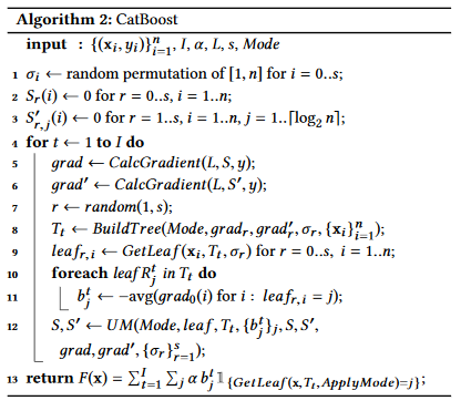
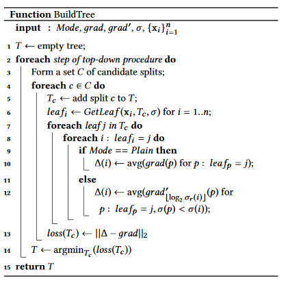
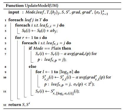
CatBoost is an algorithm for gradient boosting on decision trees. Developed by Yandex researchers and engineers, it is the successor of the MatrixNet algorithm that is widely used within the company for ranking tasks, forecasting and making recommendations. It is universal and can be applied across a wide range of areas and to a variety of problems such as search, recommendation systems, personal assistant, self-driving cars, weather prediction and many other tasks. It is in open-source and can be used by anyone now.
CatBoost is based on gradient boosted decision trees. During training, a set of decision trees is built consecutively. Each successive tree is built with reduced loss compared to the previous trees.
The number of trees is controlled by the starting parameters. To prevent over-fitting, use the over-fitting detector. When it is triggered, trees stop being built.
Before learning, the possible values of objects are divided into disjoint ranges (
Quantization is also used to split the label values when working with categorical features. А random subset of the dataset is used for this purpose on large datasets.
Two critical algorithmic advances introduced in CatBoost are the implementation
of ordered boosting, a permutation-driven alternative to the classic algorithm, and
an innovative algorithm for processing categorical features. Both techniques were
created to fight a prediction shift caused by a special kind of target leakage present
in all currently existing implementations of gradient boosting algorithms.
The most widely used technique which is usually applied to low-cardinality categorical features
is one-hot encoding; another way to deal with categorical features is to compute some statistics using the label values of the examples.
Namely, assume that we are given a dataset of observations $D = {(\mathrm{X}i, \mathrm{Y}i)\mid i=1,2,\cdots, n}$,
where $\mathrm{X}i = (x{i,1}, x{i, 2}, \cdots, x{i,m})$ is a vector of
CatBoost uses a more efficient strategy which reduces overfitting and allows to use the whole dataset
for training.
Namely, we perform a random permutation of the dataset and
for each example we compute average label value for the example with the same category value placed before the given one in the permutation.
Let
where we also add a prior value
| THREE |
|---|
 |
 |
 |

- https://tech.yandex.com/catboost/
- How is CatBoost? Interviews with developers
- Reference papers of CatBoost
- CatBoost: unbiased boosting with categorical features
- Efficient Gradient Boosted Decision Tree Training on GPUs
- CatBoost:比XGBoost更优秀的GBDT算法
There are more gradient boost tree algorithms such as ThubderGBM, TencentBoost, GBDT on angle and H2o.
- ThunderGBM: Fast GBDTs and Random Forests on GPUs
- TencentBoost: A Gradient Boosting Tree System with Parameter Server
- GBDT on Angel
- Gradient Boosted Categorical Embedding and Numerical Trees
- 从结构到性能,一文概述XGBoost、Light GBM和CatBoost的同与不同
- 从决策树、GBDT到XGBoost/lightGBM/CatBoost
- ThunderGBM:快成一道闪电的梯度提升决策树
What is the alternative of gradient descent in order to combine ADMM as an operator splitting methods for numerical optimization and Boosting such as gradient boosting/extreme gradient boosting?
Can we do leaves splitting and optimization in the same stage?
The core transfer is how to change the original optimization to one linearly constrained convex optimization so that it adjusts to ADMM:
$$
\arg\min_{f_{t}\in\mathcal F}\sum_{i=1}^{n} L[y_i,\hat{y}^{(t-1)}i + f_t(x_i)] + \gamma T +\frac{\lambda}{2}{\sum}{i=1}^{T}w_i^2 \iff \fbox{???} \quad ?
$$
where
It seems attractive to me to understand the analogy between
To be more general, how to connect the numerical optimization methods such as fixed pointed iteration methods and the boosting algorithms?
Is it possible to combine
- OPTIMIZATION BY GRADIENT BOOSTING
- boosting as optimization
- Boosting, Convex Optimization, and Information Geometry
- Generalized Boosting Algorithms for Convex Optimization
- Survey of Boosting from an Optimization Perspective
| Boosting | Optimziation |
|---|---|
| AdaBoost | Coordinate-wise Descent |
| Stochastic Gradient Boost | Stochastic Gradient Descent |
| Gradient Boost | Gradient Descent |
| Accelerated Gradient Boosting | Accelerated Gradient Descent |
| xGBoost | Newton's Methods |
| ? | Mirror Gradient Descent |
| ? | ADMM |
AdaBoost stepwise minimizes a function
Compared with entropic descent method, in each iteration of AdaBoost:
$$w_i\leftarrow w_i\exp[-\alpha_t(\mathrm{y}i G_t(x_i))]>0, i=1,2,\dots, N, \sum{n=1}^{N}w_n=1.$$
- Boost: Theory and Application
- 机器学习算法中GBDT与Adaboost的区别与联系是什么?
- Logistic Regression, AdaBoost and Bregman Distances
Another interesting question is how to boost the composite/multiplicative models rather than the additive model?
Let us assume the loss function
- Input
$D={ (x_i, y_i)}_{i=1}^{N}$ ;Loss function$G:\mathbb{R}^n\to\mathbb{R}$ . - Initialize the observation weights
$f_o=0, d_n^1=g^{\prime}(f_0(x_n), y_n), n=1, 2, \dots, N$ . - For
$t = 1, 2, \dots, T$ :- Train classifier on
${D, \mathbf d^t}$ and obtain hypothesis$h_t:\mathbb{X}\to\mathbb{Y}$ - Set
$\alpha_t=\arg\min_{\alpha\in\mathbb{R}}G[f_t + \alpha h_t]$ - Update
$f_{t+1} = f_t + {\alpha_t}h_t$ and$d_n^{t+1}=g^{\prime}(f_{t+1}(x_n), y_n), n=1, 2, \dots, N$
- Train classifier on
- Output
$f_T$ .
Here
- An Introduction to Boosting and Leveraging
- A Statistical Perspective on Algorithmic Leveraging
- FACE RECOGNITION HOMEPAGE
Matrix Multiplicative Weight can be considered as an ensemble method of optimization methods.
The name “multiplicative weights” comes from how we implement the last step: if the weight of the chosen object at step

Jeremy wrote a blog on this topic:
In general we have some set
$X$ of objects and some set$Y$ of “event outcomes” which can be completely independent. If these sets are finite, we can write down a table M whose rows are objects, whose columns are outcomes, and whose$i,j$ entry$M(i,j)$ is the reward produced by object$x_i$ when the outcome is$y_j$ . We will also write this as$M(x, y)$ for object$x$ and outcome$y$ . The only assumption we’ll make on the rewards is that the values$M(x, y)$ are bounded by some small constant$B$ (by small I mean$B$ should not require exponentially many bits to write down as compared to the size of$X$ ). In symbols,$M(x,y) \in [0,B]$ . There are minor modifications you can make to the algorithm if you want negative rewards, but for simplicity we will leave that out. Note the table$M$ just exists for analysis, and the algorithm does not know its values. Moreover, while the values in$M$ are static, the choice of outcome$y$ for a given round may be nondeterministic.
The
MWUAalgorithm randomly chooses an object$x \in X$ in every round, observing the outcome$y \in Y$ , and collecting the reward$M(x,y)$ (or losing it as a penalty). The guarantee of the MWUA theorem is that the expected sum of rewards/penalties of MWUA is not much worse than if one had picked the best object (in hindsight) every single round.
Theorem (from Arora et al): The cumulative reward of the MWUA algorithm is, up to constant multiplicative factors, at least the cumulative reward of the best object minus
- Matrix Multiplicative Weight (1)
- Matrix Multiplicative Weight (2)
- Matrix Multiplicative Weight (3)
- The Multiplicative Weights Update framework
- The Multiplicative Weights Update Method: a Meta Algorithm and Applications
- Nonnegative matrix factorization with Lee and Seung's multiplicative update rule
- A Combinatorial, Primal-Dual approach to Semidefinite Programs
- Milosh Drezgich, Shankar Sastry. "Matrix Multiplicative Weights and Non-Zero Sum Games".
- The Matrix Multiplicative Weights Algorithm for Domain Adaptation by David Alvarez Melis
- The Reasonable Effectiveness of the Multiplicative Weights Update Algorithm
- 拍拍贷教你如何用GBDT做评分卡
- LambdaMART 不太简短之介绍
- https://catboost.ai/news
- Finding Influential Training Samples for Gradient Boosted Decision Trees
- Efficient, reliable and fast high-level triggering using a bonsai boosted decision tree
- CERN boosts its search for antimatter with Yandex’s MatrixNet search engine tech
- MatrixNet as a specific Boosted Decision Tree algorithm which is available as a service
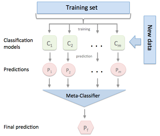
Stacked generalization (or stacking) is a different way of combining multiple models, that introduces the concept of a meta learner. Although an attractive idea, it is less widely used than bagging and boosting. Unlike bagging and boosting, stacking may be (and normally is) used to combine models of different types.
The procedure is as follows:
- Split the training set into two disjoint sets.
- Train several base learners on the first part.
- Test the base learners on the second part.
- Using the predictions from 3) as the inputs, and the correct responses as the outputs, train a higher level learner.
Note that steps 1) to 3) are the same as cross-validation, but instead of using a winner-takes-all approach, we train a meta-learner to combine the base learners, possibly non-linearly. It is a little similar with composition of functions in mathematics.
- http://www.machine-learning.martinsewell.com/ensembles/stacking/
- https://rasbt.github.io/mlxtend/user_guide/classifier/StackingClassifier/
- Stacked Generalization (Stacking)
- Stacking与神经网络 - 微调的文章 - 知乎
- http://www.chioka.in/stacking-blending-and-stacked-generalization/
- https://blog.csdn.net/willduan1/article/details/73618677
- 今我来思,堆栈泛化(Stacked Generalization)
- 我爱机器学习:集成学习(一)模型融合与Bagging
In the sense of stacking, deep neural network is thought as the stacked logistic regression. And Boltzman machine can be stacked in order to construct more expressive model for discrete random variables.
Deep Forest

- Deep forest
- https://github.com/kingfengji/gcForest
- 周志华团队和蚂蚁金服合作:用分布式深度森林算法检测套现欺诈
- Multi-Layered Gradient Boosting Decision Trees
- Deep Boosting: Layered Feature Mining for General Image Classification
- gcForest 算法原理及 Python 与 R 实现
Other ensemble methods include clustering methods ensemble, dimensionality reduction ensemble, regression ensemble, ranking ensemble.
- https://www.wikiwand.com/en/Ensemble_learning
- https://www.toptal.com/machine-learning/ensemble-methods-machine-learning
- https://machinelearningmastery.com/products/
- https://blog.csdn.net/willduan1/article/details/73618677#
- http://www.scholarpedia.org/article/Ensemble_learning
- https://arxiv.org/abs/1505.01866