Decision tree is popular and there are many free and open implementation of tree-based algorithms:
- scikit-garden,
- Treelite : model compiler for decision tree ensembles,
- bonsai-dt
- xgboost,
- catBoost,
- LightGBM,
- Ytk-learn
- thunderGBM.
The discussion Who invented the decision tree? gives some clues of the history of decision tree. Like deep learning, it has a long history.
Decision tree holds some attractive properties:
- hierarchical representation for us to understand its hidden structure;
- inherent adaptive computation;
- logical expression implementation.
Observe that we train and prune a decision tree according to a specific training data set while we representation decision tree as a collection of logical expression.
CART in statistics is a historical review on decision tree.
- Recursive Partitioning and Tree-based Methods
- https://medicine.yale.edu/profile/heping_zhang/
- https://www.stat.berkeley.edu/~breiman/RandomForests/

Now consider how to determine the structure of the decision tree.
Even for a fixed number of nodes in the tree, the problem of determining the optimal structure
(including choice of input variable for each split as well as the corresponding thresholds)
to minimize the sum-of-squares error is usually computationally infeasible
due to the combinatorially large number of possible solutions.
Instead, a greedy optimization is generally done by starting with a single root node,
corresponding to the whole input space, and then growing the tree by adding nodes one at a time.
At each step there will be some number of candidate regions in input space that can be split,
corresponding to the addition of a pair of leaf nodes to the existing tree.
For each of these, there is a choice of which of the
Note that
Note that
The decision tree is really a discriminant model
Note that the tree structure is a special type of directed acyclic graph structure. Here we focus on the connection between the decision trees and probabilistic graphical models.
Regression trees and soft decision trees are extensions of the decision tree induction technique, predicting a numerical output, rather than a discrete class.
For simplicity, we suppose that all variables are numerical and the decision tree can be expressed in a polynomials form:
The product of step functions is the indicator functions.
For example,
For categorical variables equalsto(==) test, i.e., if the variable
In MARS, the recursive partitioning regression, as binary regression tree, is viewed in a more conventional light as a stepwise regression procedure:
Delta Function is the derivative of step function, an example of generalized function;
the unit step function is the derivative of the Ramp Function defined by
Kronecker Delta is defined as
$$\delta_{ij}=\begin{cases}1, \text{if
The indicator functions is defined as $$\mathbb{1}_{ {condition} }=\begin{cases}1, &\text{if condition is hold }\ 0, &\text{otherwise}.\end{cases}$$
Given a subset characteristic function
A simple function is a finite sum
The fundamental limitation of decision tree includes:
- its lack of
continuity, - lack
smooth [decision boundary]or axe-aligned splits, - inability to provide good approximations to certain classes of simple often-occurring functions,
- highly instability with respect to minor perturbations in the training data.
The decision tree is simple function essentially.
Based on above observation, decision tree is considered to project the raw data into distinct decision region in an adaptive approach
and select the mode of within-node samples ground truth as their label.
We can replace the unit step function with truncated power series as in MARS to tackle the discontinuity to invent continuos models with continuous derivatives.
MARS is an extension of recursive partitioning regression:
Note that
There is no transformation of raw input. The decision tree is just to guide the input to a proper terminal nodes associated with some specific tests.
It is difficult to imply some properties of the input according to the test results.
To classify a new instance, one starts at the top node and applies sequentially the dichotomous tests encountered to select the
appropriate successor.
Finally, a unique path is followed, a unique terminal node is reached and the output estimation stored there is assigned to this instance.
Note that
- https://www.cs.stonybrook.edu/people/faculty/XianfengGu
- https://arxiv.org/pdf/math/0105047.pdf
- https://www3.cs.stonybrook.edu/~gu/software/manifold_spline/index.html
- https://www.ricam.oeaw.ac.at/files/reports/15/rep15-18.pdf
- https://projecteuclid.org/download/pdf_1/euclid.aos/1031594728
The MARS overcomes the (1) and (3); The fuzzy decision tree overcomes the last one. The above methods are only for regression tasks. From now we turn to the classification tasks.
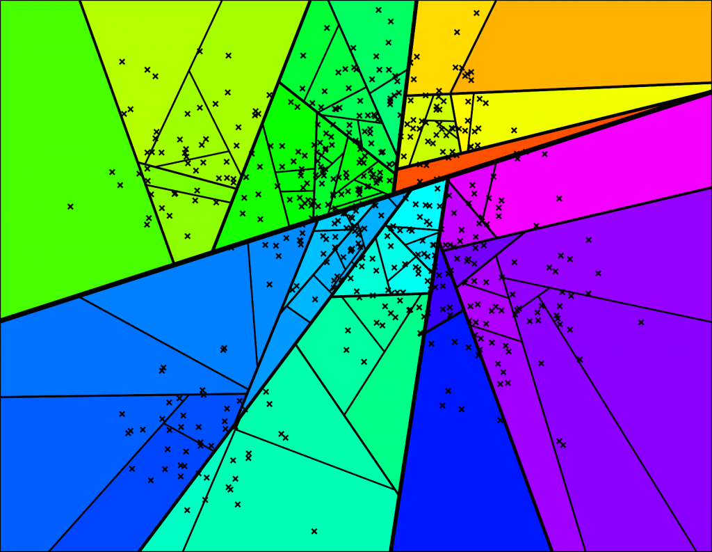
As shown in decision boundary,
In general, a pattern classifier carves up (or tesselates or partitions) the feature space into volumes called
decision regions. All feature vectors in a decision region are assigned to the same category. The decision regions are often simply connected, but they can be multiply connected as well, consisting of two or more non-touching regions.
The decision regions are separated by surfaces called the
decision boundaries. These separating surfaces represent points where there are ties between two or more categories.
The Manifold Hypothesis states that real-world high-dimensional data lie on low-dimensional manifolds embedded within the high-dimensional space, namely natural high dimensional data concentrates close to a low-dimensional manifold.
Cluster hypothesis in information retrieval is to say that documents in the same cluster behave similarly with respect to relevance to information needs.
The key idea behind the unsupervised learning of disentangled representations is that real-world data is generated by a few explanatory factors of variation which can be recovered by unsupervised learning algorithms.
- The Cluster Hypothesis: A Visual/Statistical Analysis
- https://ie.technion.ac.il/~kurland/clustHypothesisTutorial.pdf
- https://muse.jhu.edu/article/20058/pdf
- http://colah.github.io/posts/2014-03-NN-Manifolds-Topology/
- Challenging Common Assumptions in the Unsupervised Learning of Disentangled Representations
The success of decision trees is a strong evidence that both hypotheses are true.
The goal of deep learning is to learn the manifold structure in data and the probability distribution associated with the manifold.
From this geometric perspective, the unsupervised learning is to find certain properties of the manifold structure in data,
such as the Intrinsic Dimension.
What is the goal of regression tree from this geometric perspective?
Is the goal of classification tree to probability distribution associated with the manifold from this geometric perspective?
- http://www.mit.edu/people/mitter/publications/C50_sample_complexity.pdf
- http://www.mit.edu/~mitter/publications/121_Testing_Manifold.pdf
- Geometric Understanding of Deep Learning
- http://web.mit.edu/cocosci/Papers/man_nips.pdf
- Topology and Data
- UMAP: Uniform Manifold Approximation and Projection for Dimension Reduction
- https://www.krishnaswamylab.org/
- http://www.vision.jhu.edu/assets/ElhamifarNIPS11.pdf
- http://www.cs.virginia.edu/~jdl/bib/manifolds/souvenir05.pdf
- SemiBoost: Boosting for Semi-supervised Learning
- https://alexgkendall.com/media/papers/alex_kendall_phd_thesis_compressed.pdf
In some sense, a good classifier can describe the decision boundary well. And classification is connected with the manifold approximation. In practice, the problem is that the attributes are of diverse types. Although categorical attributes can be embedded into real space, it is always different to deal with categorical values and numerical values.
The decision boundary of decision trees is axis-aligned and therefor not smooth.
In fact, the product
The axis-aligned decision boundary restricts the expressivity of decision tree , which can be solved by data preprocessing and feature transformation such as kernel technique. Or we can modify the unit step function.
Template Matching is a natural approach to pattern classification. This can be done in a couple of equivalent ways:
- Count the number of agreements. Pick the class that has the maximum number of agreements. This is a maximum correlation approach.
- Count the number of disagreements. Pick the class with the minimum number of disagreements. This is a minimum error approach.
Template matching works well when the variations within a class are due to "additive noise." Clearly, it works for this example because there are no other distortions of the characters -- translation, rotation, shearing, warping, expansion, contraction or occlusion. It will not work on all problems, but when it is appropriate it is very effective. It can also be generalized in useful ways.
Template matching can easily be expressed mathematically.
Let minimum-distance classifier.
Clearly, a template matching system is a minimum-distance classifier.
If a simple minimum-distance classifier is satisfactory, there is no reason to use anything more complicated. However, it frequently happens that such a classifier makes too many errors. There are several possible reasons for this:
- The features may be inadequate to distinguish the different classes
- The features may be highly correlated
- The decision boundary may have to be curved
- There may be distinct subclasses in the data
- The feature space may simply be too complex
Linear Discriminant Analysis (LDA) is most commonly used as dimensionality reduction technique in the pre-processing step for pattern-classification and machine learning applications.
The goal is to project a dataset onto a lower-dimensional space with good class-separability in order avoid overfitting (“curse of dimensionality”) and also reduce computational costs.
LDA assumes that the observations within each class are drawn from a multivariate Gaussian distribution and the covariance of the predictor variables are common across all
Like LDA, the QDA classifier assumes that the observations from each class of Y are drawn from a Gaussian distribution. However, unlike LDA, QDA assumes that each class has its own covariance matrix.
- https://sebastianraschka.com/Articles/2014_python_lda.html
- http://washstat.org/presentations/20150604/loh_slides.pdf
- http://uc-r.github.io/discriminant_analysis
- https://pubmed.ncbi.nlm.nih.gov/12365038/
The boundaries can often be approximated by linear ones connected
by a low-dimensional nonlinear manifold.
while it is difficult to determine the number of linear approximations and their `convergence region'.
For example, we can use the multiple linear combination of features to substitute the univariate function:
We will generalize the decision boundary into decision manifold.
As decision tree consists of several leaves where k-nearest neighbor classifier perform the actual classification task by a voting scheme, model selection is related to tree technique.
The goal of decision manifold is to approximate the decision boundaries rather than the data points using similar techniques like local approximation as manifold learning.
This algorithm is based upon Self-Organizing Maps and linear classification.
Mathematically, a decision surface is a hyper-surface (i.e. of
dimension
The Decision Manifold consists of
The representatives
- The data samples are assigned to the closest local classifier representative
as the Template Matching. And compute data centroid
$n_j$ of the partition$j$ . - Once all the samples have been assigned, it is to test if samples of both classes are present at certain partition.
- If true, a linear classifier is trained for the partition
$j$ to obtain a separating hyperplane$\tilde{w}_j$ . - compute a new preliminary representative and store the information for classification in the normalized vector:
$$c_j^{\prime}=\pi_{\tilde{w}_j}(n_J), v_j^{\prime}=\frac{\tilde{w}_j}{|\tilde{w}_j|}$$ - where
$\pi_{\tilde{w}_j}(\cdot)$ denotes orthogonal projection onto the hyperplane specified by$\tilde{w}_j$
- If true, a linear classifier is trained for the partition
- Updated local classifiers subjected to the neighborhood kernel smoothing and weighted according to topological distance.
In its most simple form, classification is performed by assigning a data sample to its closest linear classifier in the same way as during training, and
then classifying it according to its position relative to the hyperplane, and is defined as
we recapitulate the properties of this method:
- The algorithm is a stochastic supervised learning method for two-class problems.
- Computation is very efficient.
- The topology induced by adjacency matrix
$A$ defines the ordering and alignment of the local classifiers; it is also exploited for optimizing classification accuracy by a weighted voting scheme. - As the topology of the decision hyper-surface is unknown, we apply a heuristic model selection that trains several classifiers with different topologies.
- The classifier performs well in case of multiple noncontiguous decision surfaces and non-linear classification problems such as XOR.
It is not a recursive partitioning method because the number of local classifiers are set as a hyperparameter determined before the training.
- http://www.ifs.tuwien.ac.at/~andi/publications/pdf/dit_ijcnn05.pdf
- http://www.ifs.tuwien.ac.at/~poelzlbauer/publications/Poe05IJCNN.pdf
- https://www.sba-research.org/team/andreas-rauber/
A natural modification is to make the step function continuous such as MARS. However, MARS is still of axis-aligned type basis expansion.
- https://astrostatistics.psu.edu/
- https://gladys-c-lipton.org/hierarchical-model/
- http://www-stat.wharton.upenn.edu/~edgeorge/
- https://bayesball.github.io/BOOK/bayesian-hierarchical-modeling.html
- https://cosx.org/2019/10/bayesian-multilevel-model/
- https://astrostatistics.psu.edu/RLectures/hierarchical.pdf
- http://varianceexplained.org/r/hierarchical_bayes_baseball/
The fuzzy decision tree introduce membership function to replace the unit step function.
In another word, the basis function is
In soft decision trees,
the unit step function
Probabilistic Boosting-Tree is the probabilistic boosting-tree that automatically constructs a tree in which each node combines a number of weak classifiers (evidence, knowledge) into a strong classifier (a conditional posterior probability).
To find smooth decision boundary of decision tree inspired methods, another technique is to transform the data at each non-terminal node.
Adaptive Neural Trees gain the complementary benefits of neural networks and decision trees.
Competitive Neural Trees for Pattern Classification contains m-ary nodes and grows during learning by using inheritance to initialize new nodes.
- https://www.cmpe.boun.edu.tr/~ethem/files/papers/BaggingSDT_ML4HIbook.pdf
- https://www.cmpe.boun.edu.tr/~ethem/files/papers/Alper-icann18.pdf
- http://www.cs.cornell.edu/~oirsoy/softtree.html
Decision trees apply the ancient wisdom "因地制宜""因材施教" to learn from data. The problem is that we should know the the training data set well and we should evaluate how well our model fit the training data set correctly. Usually the statistical prediction methods are discriminant or generative. Although the decision trees are unified in conditional framework such as Torsten Hothorn, Kurt Hornik & Achim Zeileis, it is also possible to apply tree related methods to estimate the density of the data.
- Naive Bayes, Discriminant Analysis and Generative Methods
- Comparison of Discriminant Analysis and Decision Trees for the Detection of Subclinical Keratoconus
It is natural to extend the decision boundary to piece-wise polynomial.
B-spline and Bézier Curve can be used to describe the decision boundary.
Observe that
- http://blog.pluskid.org/?p=533
- Explaining The Success Of Nearest Neighbor Methods In Prediction
- Think Globally, Fit Locally: Unsupervised Learning of Low Dimensional Manifolds
The ideal model is to learn the manifold structure of data automatically.
- https://eeecon.uibk.ac.at/~zeileis/blog/
- https://arxiv.org/pdf/1909.00900.pdf
- The power of unbiased recursive partitioning
- Unbiased Recursive Partitioning I: A Non-parametric Conditional Inference Framework
- http://www.saedsayad.com/docs/gbm2.pdf
- http://www.saedsayad.com/author.htm
- https://epub.ub.uni-muenchen.de/
We carry the integration of parametric models into trees one step further and provide a rigorous theoretical foundation by introducing a new unified framework that embeds recursive partitioning into statistical model estimation and variable selection.
Generalized linear mixed-effects model tree (GLMM tree) algorithm allows for the detection of treatment-subgroup interactions while accounting for the clustered structure of a dataset:
where
- Model-based Recursive Partitioning
- MPT trees published in BRM
- Spatial lag model trees
- Generalised Linear Model Trees with Global Additive Effects
- Partially additive (generalized) linear model trees
- party: A Laboratory for Recursive Partytioning
- https://papers.ssrn.com/sol3/papers.cfm?abstract_id=1906005
- Distributional regression forests on arXiv
- Network model trees
- Network Model Trees project
- Generalized structured additive regression based on Bayesian P-splines
- GLMM trees published in BRM
- https://eeecon.uibk.ac.at/~zeileis/news/bamlss/
In representation learning it is often assumed that real-world observations
The key idea behind this model is that the high-dimensional data
- https://www2.stat.duke.edu/~scs/Projects/Trees/BayesianCART/
- https://stat.duke.edu/people/yuhong-wu
- https://github.com/jbisbee1/BARP
- http://www.jamesbisbee.com/research/
- https://www.researchgate.net/scientific-contributions/7491056_W_J_Krzanowski
- http://users.stat.ufl.edu/~jhobert/BayesComp2020/Conf_Website/
- http://www-stat.wharton.upenn.edu/~edgeorge/
- http://www.matthewpratola.com/
- https://github.com/UBS-IB/bayesian_tree
- https://cran.r-project.org/web/packages/BayesTree/index.html
- http://www.matthewpratola.com/research/
- https://www.vanderschaar-lab.com/publications/
- Special Topics in Uncertainty Quantification via Tree-based Models and Approximate Computations
- https://pubmed.ncbi.nlm.nih.gov/29275896/
- Interpretability of Bayesian Decision Trees Induced from Trauma Data
Suppose that we have
Here we follow the framework in Recursive Partitioning and Applications. Random forest is generated in the following way:
- Draw a bootstrap sample. Namely, sample
$n$ observations with replacement from the original sample. - Apply recursive partitioning to the bootstrap sample. At each node,
randomly select
$q$ of the$p$ predictors and restrict the splits based on the random subset of the$q$ variables. Here,$q$ should be much smaller than$p$ . - Let the recursive partitioning run to the end and generate a tree.
- Repeat Steps 1 to 3 to form a forest. The forest-based classification
is made by
majority votefrom all trees.
If Step 2 is skipped, the above algorithm is called bagging (bootstraping and aggregating).
- https://www.stat.berkeley.edu/~breiman/wald2002-1.pdf
- Interpreting random forest classification models using a feature contribution method
- iterative Random Forests to discover predictive and stable high-order interactions
- Building more accurate decision trees with the additive tree
Different from random forest and bagging, boosting is aimed to find the better model via combining weaker models.
- Apply recursive partitioning to the training set and and generate a tree., wholely or partially.
- Depending on the training set errors of this predictor, change the weights and grow the next predictor.
- Repeat Steps 1 to 2 to form a forest. The forest-based classification
is made by
majority votefrom all trees.
In forest construction, there are some practical questions including the number of trees, the number of predictors, the way to train a tree.
- https://scikit-learn.org/stable/modules/ensemble.html#gradient-boosting
- https://jowel.gitlab.io/welbl/
- https://erwanscornet.github.io/
- https://phys.org/news/2018-03-science-machine-method-forests-trees.html
- https://zero-lab-pku.github.io/publication/
- https://kogalur.github.io/randomForestSRC/theory.html
- https://github.com/MingchaoZhu/InterpretableMLBook
- http://www.dabi.temple.edu/~hbling/8590.002/Montillo_RandomForests_4-2-2009.pdf
- https://ieeexplore.ieee.org/document/8933485
- http://web.ccs.miami.edu/~hishwaran/papers/BoostingLongitudinal_ML2016.pdf
An instance starts a path from the root node all the way down to a leaf node according to its real feature value in a single decision tree. All the instances in the training data will fall into several nodes and different nodes have quite different label distributions of the instances in them in the additive tree models. Every step after passing a node, the probability of being the positive class changes with the label distributions. All the features along the path contribute to the final prediction of a single tree.
There is a trend to find a balance between the accuracy and explanation by combining decision trees and deep neural networks.
The main difference from the soft decision trees are that they are designed to learn the representation of the input samples.
Instead of combining neural networks and decision trees explicitly, several works borrow ideas from decision trees for neural networks and vice versa. These models are so-called neural decision tree in this context.
Generally speaking, tree means that the instances would take different processing methods according to their feature values.
One drawback of decision tree is the lack of feature transformation.
Neural-Backed Decision Trees (NBDT) are the first to combine interpretability of a decision tree with accuracy of a neural network.
Training an NBDT occurs in 2 phases: First, construct the hierarchy for the decision tree. Second, train the neural network with a special loss term. To run inference, pass the sample through the neural network backbone. Finally, run the final fully-connected layer as a sequence of decision rules.
- Construct a hierarchy for the decision tree, called the Induced Hierarchy.
- This hierarchy yields a particular loss function, which we call the Tree Supervision Loss.
- Start inference by passing the sample through the neural network backbone. The backbone is all neural network layers before the final fully-connected layer.
- Finish inference by running the final fully-connected layer as a sequence of decision rules, which we call
Embedded Decision Rules. These decisions culminate in the final prediction.
- http://nbdt.alvinwan.com/
- https://arxiv.org/pdf/2004.00221.pdf
- Making decision trees competitive with neural networks on CIFAR10, CIFAR100, TinyImagenet200, Imagenet
- Making Decision Trees Accurate Again: Explaining What Explainable AI Did Not
Deep Neural Decision Trees (DNDT) are tree models which are realised by neural networks. A DNDT is intrinsically interpretable, as it is a tree. Yet as it is also a neural network (NN), it can be easily implemented in NN toolkits, and trained with gradient descent rather than greedy splitting.
A soft binning function is used to make the split decisions in DNDT. Given our binning function, the key idea is to construct the decision tree via Kronecker product.
- https://github.com/wOOL/DNDT
- https://arxiv.org/abs/1806.06988
- https://github.com/Nicholasli1995/VisualizingNDF
- https://sites.google.com/view/whi2018/home
- http://www.deeplearningpatterns.com/doku.php?id=deep_neural_decision_tree
Deep neural networks and decision trees operate on largely separate paradigms; typically, the former performs representation learning with pre-specified architectures, while the latter is characterised by learning hierarchies over pre-specified features with data-driven architectures. We unite the two via adaptive neural trees (ANTs), a model that incorporates representation learning into edges, routing functions and leaf nodes of a decision tree, along with a backpropagation-based training algorithm that adaptively grows the architecture from primitive modules (eg, convolutional layers).
- https://topos-theory.github.io/deep-neural-decision-forests/
- http://www.robots.ox.ac.uk/~tvg/publications/talks/deepNeuralDecisionForests.pdf
- https://www.microsoft.com/en-us/research/publication/adaptive-neural-trees/
- Deep Neural Decision Forests
- https://github.com/Microsoft/EdgeML/wiki/Bonsai
- https://www.microsoft.com/en-us/research/publication/resource-efficient-machine-learning-2-kb-ram-internet-things/
DeepGBM integrates the advantages of the both NN and GBDT by using two corresponding NN components:
(1) CatNN, focusing on handling sparse categorical features.
(2) GBDT2NN, focusing on dense numerical features with distilled knowledge from GBDT.


- Implementation for the paper "DeepGBM: A Deep Learning Framework Distilled by GBDT for Online Prediction Tasks"
- https://tracholar.github.io/wiki/machine-learning/deep-gbm.html
- http://www.arvinzyy.cn/2019/08/13/kdd-2019-paper-notes/
- DeepGBM: A Deep Learning Framework Distilled by GBDT for Online Prediction Tasks
- https://www.msra.cn/zh-cn/news/features/kdd-2019
- Unpack Local Model Interpretation for GBDT
- Optimal Action Extraction for Random Forests and Boosted Trees
- https://github.com/benedekrozemberczki/awesome-gradient-boosting-papers
Deep neural network models usually make an effort to learn a new feature space and employ a multi-label classifier on the top.
Deep Forest is an alternative of deep learning.

gcForest is the first deep learning model
which is NOT based on NNs
and which does NOT rely on BP.
- http://www.lamda.nju.edu.cn/code_gcForest.ashx
- Talk: Deep Forest Towards An Alternative to Deep Neural Networks
Different multi-label forests are ensembled in each layer of MLDF.
From layer
The critical idea of measure-aware feature reuse is to partially reuse the better representation in the previous layer on the current layer if the confidence on the current layer is lower than a threshold determined in training. Therefore, the challenge lies in defining the confidence of specific multi-label measures on demand.
- https://explainai.net/
- Deep Residual Decision Making
- Challenging Common Assumptions in the Unsupervised Learning of Disentangled Representations
- https://www.compstat.statistik.uni-muenchen.de/publications/
- Deep Embedding Forest: Forest-based Serving with Deep Embedding Features
- Multi-Label Learning with Deep Forest
- Talk: An exploration to non-NN deep models based on non-differentiable modules
Let
- H-Softmax essentially replaces the flat softmax layer with a hierarchical layer that has the words as leaves.
- Hierarchical softmax is an alternative to the softmax in which the probability of any one outcome depends on a number of model parameters that is only logarithmic in the total number of outcomes.
- Suppose we could construct a tree structure for the entire corpus, each leaf in the tree represents a word from the corpus. We traverse the tree to compute the probability of a word. The probability of each word will be the product of the probability of choosing the branch that is on the path from the root to the word.
Hierarchical softmax provides an alternative model for the conditional distributions

- https://rohanvarma.me/Word2Vec/
- Distributed Representations of Words and Phrases and their Compositionality
- Incrementally Learning the Hierarchical Softmax Function for Neural Language Models
- Softmax Regression Revisit
- http://www.hankcs.com/nlp/word2vec.html#respond
- https://arxiv.org/pdf/1402.3722v1.pdf
- https://www.iro.umontreal.ca/~lisa/pointeurs/hierarchical-nnlm-aistats05.pdf
Recursive partitioning is a very simple idea for clustering. It is the inverse of hierarchical clustering. This article provides an introduction to recursive partitioning techniques; that is, methods that predict the value of a response variable by forming subgroups of subjects within which the response is relatively homogeneous on the basis of the values of a set of predictor variables. Recursive partitioning are essentially fairly simple nonparametric techniques for prediction and classification. When used in the standard way, they provide trees which display the succession of rules that need to be followed to derive a predicted value or class. This simple visual display explains the appeal to decision makers from many disciplines. Recursive partitioning methods have become popular and widely used tools for non-parametric regression and classification in many scientific fields.
It works by building a forest of
In each tree, the set of training points is recursively partitioned into smaller and smaller subsets until a leaf node of at most M points is reached. Each partition is based on the cosine of the angle the points make with a randomly drawn hyperplane: points whose angle is smaller than the median angle fall in the left partition, and the remaining points fall in the right partition.
The resulting tree has predictable leaf size (no larger than M) and is approximately balanced because of median splits, leading to consistent tree traversal times.
Querying the model is accomplished by traversing each tree to the query point's leaf node to retrieve ANN candidates from that tree, then merging them and sorting by distance to the query point.
- https://github.com/lyst/rpforest
- https://ibex.readthedocs.io/en/latest/api_ibex_sklearn_neighbors_lshforest.html
- https://github.com/spotify/annoy
- https://www.ilyaraz.org/
- https://www.ilyaraz.org/static/papers/phd_thesis.pdf
We present such a method for multi-dimensional image compression called Compression via Adaptive Recursive Partitioning (CARP). In Nearest Neighbor Search, recursive partitioning is referred as an approximate methods related with k-d tree as shown in Nearest neighbors and vector models – part 2 – algorithms and data structures.
Nice! We end up with a binary tree that partitions the space.
The nice thing is that points that are close to each other in the space are more likely to be close to each other in the tree.
In other words, if two points are close to each other in the space,
it's unlikely that any hyperplane will cut them apart.
To search for any point in this space, we can traverse the binary tree from the root. Every intermediate node (the small squares in the tree above) defines a hyperplane, so we can figure out what side of the hyperplane we need to go on and that defines if we go down to the left or right child node. Searching for a point can be done in logarithmic time since that is the height of the tree.
- 14.2 - Recursive Partitioning
- Recursive Partitioning
- Recursive Partitioning and Tree-based Methods
- Metric Indexes based on Recursive Voronoi Partitioning
- CARP: Compression through Adaptive Recursive Partitioning for Multi-dimensional Images
There are many data structure based on tree such as binary tree, red-black tree, B+ tree, wavelet tree. libcds implements low-level succinct data structures such as bitmaps, sequences, permutations, etc. The main goal is to provide a set of structures that form the building block of most compressed/succinct solutions. In the near future we are planning to add compression algorithms and support for succinct trees.
- https://dev.to/frosnerd/memory-efficient-data-structures-2hki
- https://www.cs.princeton.edu/courses/archive/spr05/cos598E/
- http://www.bowdoin.edu/~ltoma/teaching/cs340/spring08/
- http://people.duke.edu/~ccc14/sta-663-2016/A04_Big_Data_Structures.html
- http://people.seas.harvard.edu/~minilek/cs229r/fall15/index.html
- http://www2.compute.dtu.dk/courses/02951/
- http://roaringbitmap.org/
- https://mrdata.usgs.gov/mrds/compact/dd.php
- https://github.com/fclaude/libcds
- https://opendsa-server.cs.vt.edu/ODSA/Books/CS3/html/
A Tree is a recursive data structure containing the set of one or more data nodes where one node is designated as the root of the tree while the remaining nodes are called as the children of the root.
In a general tree, A node can have any number of children nodes but it can have only a single parent.
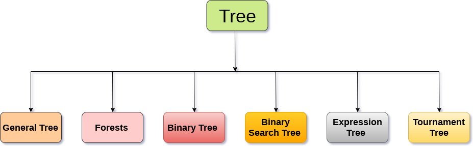
Expression treesare used to evaluate the simple arithmetic expressions. Expression tree is basically a binary tree where internal nodes are represented by operators while the leaf nodes are represented by operands. Expression trees are widely used to solve algebraic expressions like (a+b)*(a-b). Consider the following example.
In Linked Representation, the binary tree is stored in the memory, in the form of a linked list where the number of nodes are stored at non-contiguous memory locations and linked together by inheriting parent child relationship like a tree. every node contains three parts : pointer to the left node, data element and pointer to the right node. Each binary tree has a root pointer which points to the root node of the binary tree. In an empty binary tree, the root pointer will point to null.
- https://www.javatpoint.com/binary-tree
- https://www.cs.cmu.edu/~adamchik/15-121/lectures/Trees/trees.html
- http://cslibrary.stanford.edu/110/BinaryTrees.html
The sequential representation uses an array for the storage of tree elements.
The number of nodes a binary tree has defines the size of the array being used. The root node of the binary tree lies at the array’s first index. The index at which a particular node is stored will define the indices at which the right and left children of the node will be stored. An empty tree has null or 0 as its first index.
Binary Search tree can be defined as a class of binary trees, in which the nodes are arranged in a specific order. This is also called ordered binary tree.
In a binary search tree, the value of all the nodes in the left sub-tree is less than the value of the root.
Similarly, value of all the nodes in the right sub-tree is greater than or equal to the value of the root.
This rule will be recursively applied to all the left and right sub-trees of the root.
Given a list of number, we create a binary tree in the following way:
- Insert the first element into the tree as the root of the tree.
- Read the next element, if it is lesser than the root node element, insert it as the root of the left sub-tree.
- Otherwise, insert it as the root of the right of the right sub-tree.
- https://www.javatpoint.com/binary-search-tree
- https://www.topcoder.com/community/competitive-programming/tutorials/an-introduction-to-binary-search-and-red-black-trees/
AVL Tree can be defined as height balanced binary search tree in which each node is associated with a balance factor which is calculated by subtracting the height of its right sub-tree from that of its left sub-tree.
AVL tree controls the height of the binary search tree by not letting it to be skewed. The time taken for all operations in a binary search tree of height h is
- https://www.javatpoint.com/avl-tree
- https://www.programiz.com/dsa/avl-tree
- https://planetlotus.github.io/2020/06/14/algorithm-visualizer-avl-tree-part-1.html
- https://visualgo.net/en/bst
- https://www.cs.auckland.ac.nz/software/AlgAnim/AVL.html
- https://bradfieldcs.com/algos/trees/avl-trees/
B Tree is a specialized m-way tree that can be widely used for disk access. A B-Tree of order m can have at most m-1 keys and m children. One of the main reason of using B tree is its capability to store large number of keys in a single node and large key values by keeping the height of the tree relatively small.
A B tree of order m contains all the properties of an M way tree. In addition, it contains the following properties.
- Every node in a B-Tree contains at most m children.
- Every node in a B-Tree except the root node and the leaf node contain at least m/2 children.
- The root nodes must have at least 2 nodes.
- All leaf nodes must be at the same level.
It is not necessary that, all the nodes contain the same number of children but, each node must have m/2 number of nodes.
A B-tree is a tree data structure that keeps data sorted and allows searches, insertions, and deletions in logarithmic amortized time. Unlike self-balancing binary search trees, it is optimized for systems that read and write large blocks of data. It is most commonly used in database and file systems.
B+ Tree is an extension of B Tree which allows efficient insertion, deletion and search operations.
In B Tree, Keys and records both can be stored in the internal as well as leaf nodes. Whereas, in B+ tree, records (data) can only be stored on the leaf nodes while internal nodes can only store the key values.
- https://www.javatpoint.com/b-plus-tree
- http://www.cburch.com/cs/340/reading/btree/index.html
- http://blog.codinglabs.org/articles/theory-of-mysql-index.html
Spatial Trees are a recursive space partitioning data structure that can help organize high-dimensional data.
They can assist in analyzing the underlying data density,
perform fast nearest-neighbor searches,
and do high quality vector-quantization.
There are several instantiations of spatial trees.
The most popular include KD trees, RP trees (random projection trees), PD trees (principal direction trees).
- https://www.ilyaraz.org/static/class_2018/
- https://github.com/rpav/spatial-trees
- https://www.cliki.net/spatial-trees
- http://www.sai.msu.su/~megera/
- http://ann-benchmarks.com/
- https://zilliz.com/cn/
- https://www.milvus.io/
- http://www.cs.cmu.edu/~agray/nbody.html
- http://cseweb.ucsd.edu/~naverma/SpatialTrees/index.html
- https://www.cs.ubc.ca/~nando/nipsfast/slides/gray.pdf
- https://www1.cs.columbia.edu/CAVE/projects/search/
- https://www.cs.princeton.edu/courses/archive/spr05/cos598E/bib/p208-lv.pdf

Random Projection Trees is a recursive space partitioning datastructure which can automatically adapt to the underlying (linear or non-linear) structure in data. It has strong theoretical guarantees on rates of convergence and works well in practice.
You can use RPTrees to learn the structure of manifolds, perform fast nearest-neighbor searches, do vector-quantization of the underlying density, and much more.
- http://cseweb.ucsd.edu/~naverma/RPTrees/publication.html
- http://cseweb.ucsd.edu/~naverma/RPTrees/tutorial.html
- https://theory.cs.washington.edu/
- Random projection trees and low dimensional manifolds
- Random Projections of Smooth Manifolds
- Fast Nearest Neighbor Search through Sparse Random Projections and Voting
- http://cseweb.ucsd.edu/~dasgupta/papers/exactnn-algo.pdf
- https://sourceforge.net/projects/rptree/
- https://cseweb.ucsd.edu/~dasgupta/papers/vq.pdf
- http://jmlr.csail.mit.edu/papers/volume21/18-664/18-664.pdf
The NV-tree is a disk-based data structure, which builds upon a combination of projections of data points to lines and partitioning of the projected space. By repeating the process of projecting and partitioning, data is eventually separated into small partitions which can easily be fetched from disk with a single disk read, and which are highly likely to contain all the close neighbors in the collection. In this thesis we develop the NVtree as a full-fledged database solution, addressing all three requirements of scalability, dynamicity and durability.

- https://fribbels.github.io/vptree/writeup
- http://pages.cs.wisc.edu/~mcollins/software/vptree.html
- http://stevehanov.ca/blog/index.php?id=130
- https://www.researchgate.net/publication/221636690_VP-tree_Content-Based_Image_Indexing
- https://www.pyimagesearch.com/2019/08/26/building-an-image-hashing-search-engine-with-vp-trees-and-opencv/
With the availability of large databases and recent improvements in deep learning methodology, the performance of AI systems is reaching, or even exceeding, the human level on an increasing number of complex tasks.
Impressive examples of this development can be found in domains such as image classification, sentiment analysis, speech understanding or strategic game playing.
However, because of their nested non-linear structure, these highly successful machine learning and artificial intelligence models are usually applied in a black-box manner, i.e. no information is provided about what exactly makes them arrive at their predictions.
Since this lack of transparency can be a major drawback, e.g. in medical applications, the development of methods for visualizing, explaining and interpreting deep learning models has recently attracted increasing
attention.
The decision boundary of decision trees are clear and parameterized. The visualization, explaining and interpreting decision tree models seems muck easier than deep models.
Like geometry, there are diverse forms of decision trees:
- Graphical form;
- Logical form;
- Analytic form.
And analytic form of decision trees are close to neural network. Neural decision trees,


- https://github.com/wOOL/DNDT
- Interpretable Decision Sets: A Joint Framework for Description and Prediction
- http://yosinski.com/deepvis
- https://sites.google.com/corp/view/whi2018
- http://airesearch.com/
- http://www.ise.bgu.ac.il/faculty/liorr/
- Decision Forests for Computer Vision and Medical Image Analysis
- EXPLAINABLE ARTIFICIAL INTELLIGENCE
- Interpretable Machine Learning
- https://christophm.github.io/interpretable-ml-book/
- https://beenkim.github.io/
- https://zhuanlan.zhihu.com/p/78822770
- https://zhuanlan.zhihu.com/p/74542589
- https://www.jiqizhixin.com/articles/0211
- https://www.unite.ai/what-is-a-decision-tree/
- https://github.com/conan7882/CNN-Visualization
- https://kogalur.github.io/randomForestSRC/index.html
The recommender system is different from search because there is no explicit query in the recommender system. The recommender learn the users' preference or interest in some items under some specific context. In an abstract way, the recommender system is to map the information of the user into the sorted order of the items.
We have shown that the essence of the decision tree is template matching. Tree-based techniques can speed up the search of items such as the vector search model.
- https://www.infoq.cn/article/y95dtkfr2_lhBus40Ksi
- https://blog.csdn.net/b0Q8cpra539haFS7/article/details/79722374
- https://arxiv.org/pdf/1902.07565.pdf
- https://github.com/imsheridan/DeepRec
- https://arxiv.org/abs/1801.02294
- https://github.com/LRegan666/Tree_Deep_Model
Many multiple adaptive regression methods are specializations of a general multivariate
regression algorithm that builds hierarchical models using a set of basis
functions and stepwise selection:
Let us compare hierarchical models including decision tree, multiple adaptive regression spline and Recursive partitioning regression.
| Decision Tree | MARS | Multivariate adaptive polynomial synthesis (MAPS) |
|---|---|---|
| Discontinuity | Smoothness | ---- |
| Unit step function | ReLU |
The sum-product network is the general form in Tractable Deep Learning.
Essentially all tractable graphical models can be cast as SPNs, but SPNs are also strictly more general. We then propose learning algorithms for SPNs, based on backpropagation and EM.
The compactness of graphical models can often be greatly
increased by postulating the existence of hidden variables
The SPN is defined as following
A SPN is rooted DAG whose leaves are
$x_1, \cdots , x_n$ and $\bar{x}_1, \cdots, \bar{x}n$ with internal sum and product nodes, where each edge $(i, j)$ emanating from sum node $i$ has a weight $w{i} \geq 0$.
Advantages of SPNs:
- Unlike graphical models, SPNs are tractable over high treewidth models
- SPNs are a deep architecture with full probabilistic semantics
- SPNs can incorporate features into an expressive model without requiring approximate inference.
Decision tree is flexible with categorical and numerical variable. Besides the dummy variables, another generalization of decision tree is the statistical relational learning based on sum-product network.
Conventional machine learning techniques have two primary assumptions that limit their application in relational domains.
First, algorithms for propositional data assume that data instances are recorded in homogeneous structures (i.e., a fixed number of attributes for each entity) but relational data instances are usually more varied and complex (e.g., molecules have different numbers of atoms and bonds).
Second, the algorithms assume that data instances are independent but relational data often violate this assumption---dependencies may occur either as a result of direct relations or through chaining multiple relations together.
For example, scientific papers have dependencies through both citations (direct) and authors (indirect).
- Introduction to Statistical Relational Learning
- https://data-science-blog.com/blog/2016/08/17/statistical-relational-learning/
- https://martint.blog/
- Robert Peharz publication
- Talk: Tractable Models and Deep Learning: A Love Marriage (Robert Peharz)
- http://www.stat.yale.edu/~arb4/publications.html
Pairwise Learning refers to learning tasks with the associated loss functions depending on pairs of examples.
Circle Loss provides a pair similarity optimization viewpoint on deep feature learning, aiming to maximize the within-class similarity
Optimizing unified loss function is defined as
$$\mathcal{L}{uni}(x)=\log[1+\exp(\sum{i}\sum_{j}\gamma((s_n^j − s_p^i+m)))]$$
in which
We consider to enhance the optimization flexibility by allowing each similarity score to learn at its own pace, depending on its current optimization status.
The unified loss function is transferred into the proposed Circle loss by
$$\mathcal{L}{circle}(x)=\log[1+\exp(\sum{i}\sum_{j}\gamma((\alpha_p^i s_n^j − \alpha_p^i s_p^i)))]$$
in which
- Learning pairwise image similarities for multi-classification using Kernel Regression Trees
- https://arxiv.org/pdf/1612.02295.pdf
- https://arxiv.org/pdf/1703.07464.pdf
- https://www.salford-systems.com/products/mars
- MARS
- Discussion
- Tree-classifier via Nearest Neighbor Graph Partitioning
- Recursive Partitioning for Personalization using Observational Data
- https://statmodeling.stat.columbia.edu/2019/11/26/machine-learning-under-a-modern-optimization-lens-under-a-bayesian-lens/
- https://arxiv.org/abs/1908.01755
- https://arxiv.org/abs/1904.12847
- http://akyrillidis.github.io/
————————
- https://github.com/jwasham/coding-interview-university
- https://github.com/jackfrued/Python-100-Days
- https://tlverse.org/tmle3/index.html
Contrastive methods, as the name implies, learn representations by contrasting positive and negative examples. Although not a new paradigm, they have led to great empirical success in computer vision tasks with unsupervised contrastive pre-training.
Clusters of points belonging to the same class are pulled together in embedding space, while simultaneously pushing apart clusters of samples from different classes.
More formally, for any data point
- here
$x^+$ is data point similar or congruent to$x$ , referred to as a positive sample. -
$x^-$ is a data point dissimilar to$x$ , referred to as a negative sample. - the
$\textrm{score}$ function is a metric that measures the similarity between two features.
Here the
- https://paperswithcode.com/
- https://paperswithcode.com/sota
- https://github.com/HobbitLong/SupContrast
- Supervised Contrastive Learning
- https://ankeshanand.com/blog/2020/01/26/contrative-self-supervised-learning.html
Super Learner is motivated by this use of cross validation as a weighted combination of many candidate learners.
- https://tlverse.org/tmle3/index.html
- https://tlverse.org/sl3/
- https://pubmed.ncbi.nlm.nih.gov/17910531/
Tree is a special kind of Directed Acyclic Graph.
- https://en.wikipedia.org/wiki/Network_calculus
- https://www.nps.edu/web/math/network-science
- https://www.siam.org/conferences/cm/conference/ns18
There are four key network properties to characterize a graph: degree distribution, path length, clustering coefficient, and connected components.
The connectivity of a graph measures the size of the largest connected component.
The largest connected component is the largest set where any two vertices can be joined by a path.
The clustering coefficient (for undirected graphs) measures what proportion of node
- https://github.com/GraphBLAS/graphblas-pointers
- http://graphblas.org/index.php?title=Graph_BLAS_Forum
- Graph Algorithms in the Language of Linear Algebra
- https://www.cs.yale.edu/homes/spielman/
- https://github.com/alibaba/euler
- https://ci.apache.org/projects/flink/flink-docs-stable/dev/libs/gelly/
- http://tinkerpop.apache.org/
The oridnary database stores the tabular data, where each record makes up a row like a vector. And Structured Query Language (SQL) is the standard language to query the vector-like data. And many search engines are based on the vector search.
- https://www.cnblogs.com/myitroad/p/7727570.html
- https://blog.csdn.net/javeme/article/details/82631834
- http://tinkerpop.apache.org/
A computational graph is defined as
a directed graph where the nodes correspond to mathematical operations. Computational graphs are a way of expressing and evaluating a mathematical expression.
[To create a computational graph, we make each of these operations, along with the input variables, into nodes. When one node’s value is the input to another node, an arrow goes from one to another.](- http://colah.github.io/posts/2015-08-Backprop/)
- https://deepnotes.io/tensorflow
- https://sites.google.com/a/uclab.re.kr/lhparkdeep/feeding-habits
- https://kharshit.github.io/blog/
- http://rll.berkeley.edu/cgt/
- http://www.charuaggarwal.net/
- https://www.cl.cam.ac.uk/~ey204/teaching/ACS/R244_2017_2018/presentation/S2/Nat_TF.pdf
- DEEP LEARNING WITH DYNAMIC COMPUTATION GRAPHS
One application of computational graph is to explain the automatic differentiation or auto-diff.
- http://www.autodiff.org/
- https://github.com/apache/incubator-tvm
- https://tvm.apache.org/
- https://github.com/google/jax
- https://github.com/TimelyDataflow/differential-dataflow
- http://www.optimization-online.org/DB_FILE/2020/02/7640.pdf
Decision jungles have the following advantages:
- By allowing tree branches to merge, a decision DAG typically has a lower memory footprint and a better generalization performance than a decision tree, albeit at the cost of a somewhat higher training time.
- Decision jungles are non-parametric models, which can represent non-linear decision boundaries.
- They perform integrated feature selection and classification and are resilient in the presence of noisy features.
A binary decision tree is a binary tree
- Feature dimension
$d_v \in {1,...,n}$ - Threshold
$\theta_v \in \mathbb{R}$
A leaf node
- Class label
$c_v$ - or class histogram
$h_v : {1,...,C} \to \mathbb R$ .
A data point
The idea of Decision DAG is to use a directed acyclic graph (DAG) instead of a tree graph.
A decision DAG is a directed acyclic graph
- Feature dimension
$d_v \in {1,...,n}$ ; - Threshold
$\theta_v \in \mathbb{R}$ ; - Left child node
$l_v \in V$ ; - Right child node
$r_v \in V$ .
A random decision DAG is a decision DAG whose parameters are sampled from some probability distribution. A
decision jungle$J = (G_1,...,G_m)$ is an ensemble of random decision DAGs$G_i$ .
- http://www.nowozin.net/sebastian/
- http://www.nowozin.net/sebastian/papers/shotton2013jungles.pdf
- Decision Jungles: Compact and Rich Models for Classification
- https://www.microsoft.com/en-us/research/video/decision-jungles/
- Decision Jungles: Compact and Rich Models for Classification
- http://www.mbmlbook.com/
- http://www.mbmlbook.com/MBMLbook.pdf
- http://geekstack.net/resources/public/downloads/tobias_pohlen_decision_jungles_slides.pdf
- https://bitbucket.org/geekStack/libjungle/src
- http://pdollar.github.io/toolbox/index.html
- http://geekstack.net/resources/public/downloads/tobias_pohlen_decision_jungles.pdf
The Dataflow Model is to deal with the distributed machine learning which focus on the data rather than the operation.
| Map-Reduce | Iterative Map-reduce | Parameter sever | Data flow |
|---|---|---|---|
| Hadoop | Twister | Flink | Tensorflow |
- http://iterativemapreduce.org/
- https://github.com/dmlc/ps-lite
- https://ps-lite.readthedocs.io/en/latest/
The dataflow model use the Directed Acyclic Graph (DAG) to describe the programs.
- The Dataflow Model: A Practical Approach to Balancing Correctness, Latency, and Cost in Massive-Scale, Unbounded, Out-of-Order Data Processing
- http://cs.brown.edu/~ugur/vldbj03.pdf
- https://www.cl.cam.ac.uk/~ey204/teaching/ACS/R244_2017_2018/presentation/S5/Thomas_DFM.pdf
- https://www.cl.cam.ac.uk/~ey204/teaching/ACS/R244_2017_2018/
- https://id2221kth.github.io/
- https://yq.aliyun.com/articles/64911
- https://cloud.google.com/dataflow/
- https://nifi.apache.org/index.html
- https://my.oschina.net/taogang/blog/1819665
- Awesome Flow-Based Programming (FBP) Resources
- Naiad: A Timely Dataflow System
Airflow is a platform to programmatically author, schedule and monitor workflows.
Use Airflow to author workflows as Directed Acyclic Graphs (DAGs) of tasks. The Airflow scheduler executes your tasks on an array of workers while following the specified dependencies. Rich command line utilities make performing complex surgeries on DAGs a snap. The rich user interface makes it easy to visualize pipelines running in production, monitor progress, and troubleshoot issues when needed.
Airflow is not a data streaming solution. Tasks do not move data from one to the other (though tasks can exchange metadata!).
- http://oozie.apache.org/
- http://airflow.apache.org/index.html
- https://azkaban.github.io/
- https://www.xuxueli.com/xxl-job/
- https://open-data-automation.readthedocs.io/en/latest/fme/job-scheduling.html
- https://wexflow.github.io/
- Decision Jungles: Compact and Rich Models for Classification
Graph Learning is to learn from the graph data: Simply said, it’s the application of machine learning techniques on graph-like data. Deep learning techniques (neural networks) can, in particular, be applied and yield new opportunities which classic algorithms cannot deliver.
- https://snap-stanford.github.io/cs224w-notes/machine-learning-with-networks/graph-neural-networks
- https://graphsandnetworks.com/blog/
- http://web.stanford.edu/class/cs224w/
- https://networkdatascience.ceu.edu/
- http://tensorlab.cms.caltech.edu/users/anima/
- https://graphvite.io/
- https://github.com/alibaba/graph-learn
- https://www.mindspore.cn/install
- http://www.norbertwiener.umd.edu/
- http://david-wild-knzl.squarespace.com/
- https://github.com/stanford-ppl/Green-Marl
- https://arxiv.org/abs/2001.00426
- https://sigport.org/
- https://sigport.org/sites/default/files/graphSP_prob.pdf
- http://biron.usc.edu/wiki/index.php/EE_599_Graph_Signal_Processing
- http://gspworkshop.org/
- https://lts2.epfl.ch/
- https://pygsp.readthedocs.io/en/stable/https://pygsp.readthedocs.io/en/stable/
- https://epfl-lts2.github.io/gspbox-html/
- http://2019.ieeeglobalsip.org/pages/symposium-graph-signal-processing
- http://spark.apache.org/graphx/
- http://giraph.apache.org/
- https://www.graphengine.io/
- http://web.media.mit.edu/~xdong/resource.html
- https://epfl-lts2.github.io/gspbox-html/
- https://www.usenix.org/conference/fast17/technical-sessions/presentation/liu
- https://github.com/twitter/cassovary
Linked data are special kind of graph data. For example, we not only care the components in chemistry but also their bonds.
- https://info.sice.indiana.edu/~dingying/Teaching/S604/LODBook.pdf
- http://cheminfov.informatics.indiana.edu:8080/c2b2r/
- Linked Data Glossary
- http://events.linkeddata.org/ldow2018/
- http://schlegel.github.io/balloon/
- https://www.w3.org/standards/semanticweb/data
- https://csarven.ca/linked-statistical-data-analysis
- https://www.cdc.gov/nchs/data-linkage/index.htm
- http://www.iaria.org/conferences2018/ALLDATA18.html
- https://hunglvosu.github.io/res/lect10-social-net.pdf
- https://socialnetwork.readthedocs.io/en/latest/index.html
- https://www.cs.purdue.edu/homes/neville/
- https://www.knime.com/network-mining
- https://www.knime.com/knime-labs
- http://gautambhat.github.io/gautambhat.github.io/
- http://aimlab.cs.uoregon.edu/smash/
- http://monajalal.github.io/
Graph neural networks are aimed to process the graph data with the deep learning models.
Generally, deep neural networks are aimed at the tensor inputs.
- https://grlplus.github.io/
- http://tkipf.github.io/
- Deep learning with graph-structured representations
- Natural Language Processing and Text Mining with Graph-structured Representations
- The resurgence of structure in deep neural networks
- https://nlp.stanford.edu/~socherr/thesis.pdf
- https://www.cl.cam.ac.uk/~pl219/
- https://cqf.io/papers/Dynamic_Hierarchical_Mimicking_CVPR2020.pdf
Transformers are Graph Neural Networks.
At a high level, all neural network architectures build representations of input data as vectors/embeddings, which encode useful statistical and semantic information about the data. These latent or hidden representations can then be used for performing something useful, such as classifying an image or translating a sentence.
We update the hidden feature of the $j$th word in a sentence from layer
$$\text{where} \ w_{ij} = \text{softmax}j \left( Q^{\ell} h{i}^{\ell} \cdot K^{\ell} h_{j}^{\ell} \right),$$
where