There is another trichotomy in statistics
descriptive analysis, exploratory analysis, inferential analysis.

- https://www.upstreamml.com/
- https://wid.wisc.edu/
- https://machinelearning.wisc.edu/
- https://www.merantix.com/
- https://www.l3s.de/en
- https://lucid.wisc.edu/
- https://amueller.github.io/COMS4995-s18/
- https://www.ml.uni-saarland.de/index.htm
- https://mathinvestor.org/
- https://idalab.de/
- IIS: RI: Small: Nonlinear Dynamical System Theory for Machine Learning
- Acceleration Techniques for Lower-Order Algorithms in Nonlinear Optimization
There are two different contexts in clustering, depending on how the entities to be clustered are organized.
In some cases one starts from an internal representation of each entity (typically an
The external representation of dissimilarity will be discussed in Graph Algorithm.
- http://sklearn.apachecn.org/cn/0.19.0/modules/clustering.html
- https://www.wikiwand.com/en/Cluster_analysis
- https://www.toptal.com/machine-learning/clustering-algorithms
- https://blog.csdn.net/xiaojimanman/article/details/44977889
- https://github.com/hankcs/HanLP/wiki/%E6%96%87%E6%9C%AC%E8%81%9A%E7%B1%BB
- http://www.charuaggarwal.net/text-cluster.pdf
- https://www.tutorialspoint.com/data_mining/dm_cluster_analysis.htm
- Influential features PCA for high dimensional clustering
- http://www.andrew.cmu.edu/user/davidch/
K-means is also called Lloyd algorithm. It is a prototype-based clustering method.
- Set the class number
$k$ and initialize the centers of the classes${c_i, c_2, \dots, c_k}$ .- Split the data set to
$k$ classes by the shortest distance to the center:$$\arg\min_{i}|x-c_i|$$ - Update the center of the class
$i$ :$$c_i\leftarrow \frac{\sum_{x}\mathbb{I}(x\in \text{Class i})x}{\sum_{x}\mathbb{I}(x\in \text{Class i})}$$ - Until the stop criterion is satisfied.
The indicator function
In optimization form, it is to minimize the following objective function distortion measure:
$$ J = \sum_{n=1}^{N}\sum_{k=1}^{K} \mathbb{I}{nk}|x_n-\mu_k|^2 $$ where $\mathbb{I}{nk}$ is a binary Dirac function.
After initializing the
Then we fix $\mathbb{I}{nk}$ and optimize the objective function with respect to $\mu_k$: setting $\frac{\partial J}{\partial \mu_k} = 0$, we obtain $$ \mu_k = \frac{\sum_n \mathbb{I}{nk}x_n}{\sum_n \mathbb{I}_{nk}}. $$
In the first procedure, it is supposed to maximize the inter-cluster dissimilarity; The second procedure, it is supposed to minimize the intra-cluster distance.
The loss function of K-means can be any sum of inter-cluster distance
$$D_K=\sum_{k=1}^K \text{inter-cluster distance of
Gap Statistic is defined as
And the optimal number of
In K-means, we compute the mean or average of the samples in a class to update the centroid. It is interesting to observe the "variance" or "range" of the clusters. The samples in the same cluster may be generated by the same pattern or distribution.
In statistics, the mixture distribution can describe complicated probability distribution such as Gaussian mixture model.
Suppose that the population is distributed in the mixture of Gaussian distribution:
$$
P(x) = \sum_{k=1}^{K}p(k) p(x|k)
= \sum_{k=1}^{K}\pi(k) N(x|\mu_k,\Sigma_k)
$$
where the discrete distribution of clustering
Like K-means clustering, the class number

The likelihood of the observed random variables is given by $$ \prod_{i=1}^{N} P(x_i)= \prod_{i=1}^{N} \sum_{k=1}^{K}\pi(k) N(x_i |\mu_k,\Sigma_k) $$
so that the log-likelihood function is given by $$ \log\prod_{i}^{N} P(x_i)= \sum_{i}^{N} \log[\sum_{k=1}^{K}\pi(k) N(x_i|\mu_k,\Sigma_k)]. $$
In The Nature of Statistical Learning, an example of Gaussian mixture is given which cannot be estimated via maximum likelihood estimation directly.
Bishop introduces clustering in Bayesian perspective :
An elegant and powerful method for finding maximum likelihood solutions for models with latent variables is called the expectation-maximization algorithm, or EM algorithm.
Let us begin by writing down the conditions that must be satisfied at a maximum
of the likelihood function. Setting the derivatives of log-likelihood function with
respect to the means
And if we define
where we define
And similarly, we can obtain that $$ \Sigma_k = \frac{1}{N_k}\sum_{i=1}^{N} \gamma(z_{ik}) (x_i - \mu_k)(x_i - \mu_k)^T. $$
The
By setting the derivatives to zeros, we obtain
Multiplying by inverse of matrix
- http://www.vlfeat.org/index.html
- 理解EM算法 - SIGAI的文章
- https://jakevdp.github.io/PythonDataScienceHandbook/05.12-gaussian-mixtures.html
- https://www.wikiwand.com/en/Mixture_distribution
- http://www.cnblogs.com/mingfengshan/p/6848989.html
- https://brilliant.org/wiki/gaussian-mixture-model/
- https://site.douban.com/182577/widget/notes/10567212/note/271336847/
- http://120.52.51.19/www.cs.toronto.edu/~rsalakhu/STA4273_2015/notes/Lecture5_2015.pdf
K-medoids Clustering is the twin of the k-means clustering. Rather than using conventional mean/centroid,
it uses medoids to represent the clusters. The medoid is a statistic which represents that data
member of a data set whose average dissimilarity to all the other members of the set is minimal.
Let Medoid is defined as
$$ x_{\text{medoid}} = {\arg\min}{y\in {x{1},x_{2},\cdots ,x_{n}}} \sum_{i=1}^{n} d(y,x_{i}). $$
The simplified version is to compute the median of each attribute to approximate medoid instead of the optimization in the definition, where the dissimilarity function
It also begins with randomly selecting k data items as initial medoids to represent the k clusters. All
the other remaining items are included in a cluster which has its medoid closest to them.
Thereafter a new medoid is determined which can represent the cluster better. All the remaining data items are yet again assigned to the clusters having closest medoid.
In each iteration, the medoids alter their location. The method minimizes the sum of the dissimilarities between each data item and its corresponding medoid.
This cycle is repeated till no medoid changes its
placement.
This marks the end of the process and we have the resultant final clusters with their medoids defined.
- http://www.math.le.ac.uk/people/ag153/homepage/KmeansKmedoids/Kmeans_Kmedoids.html
- http://blog.pluskid.org/?p=40
- https://wireilla.com/ns/maths/Papers/3314ijscmc01.pdf
The hard clustering problem consists of partitioning the entities
- Minimization of the average intra-cluster dissimilarities;
- Maximization of inter-cluster distance.
How can we do to choose the dissimilarities and distance?
intra-cluster dissimilarities |
inter-cluster distance |
|---|---|
| variance | differences of summary statistics |
|
|
|
| proximality/similarity | speratabilty/dissimilarity |
| ? | ? |
Iterative Self-Organizing Data Analysis Technique Algorithm(ISODATA)
- https://www.cnblogs.com/PIESat/p/10212994.html
- https://www.cnblogs.com/huadongw/articles/4101306.html
Hierarchical clustering algorithms are either top-down or bottom-up. These methods are based on the choice of distance measure or metric.
Bottom-up algorithms (Agglomerative Hierarchical Clustering) treat each document as a singleton cluster at the outset and then successively merge (or agglomerate) pairs of clusters until all clusters have been merged into a single cluster that contains all documents.
The algorithm works as follows:
- Put each data point in its own cluster.
- Identify the closest two clusters and combine them into one cluster.
- Repeat the above step until all the data points are in a single cluster.
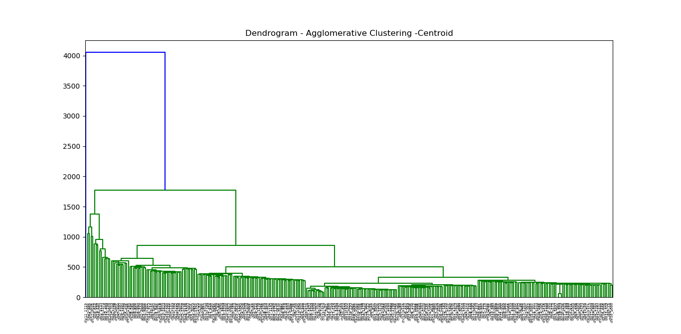
The idea is to build a binary tree of the data that successively merges similar groups of points.
And we identify the closest two clusters by the group similarity of these clusters.
There are three most popular choices of group similarity induced by a distance measure between points
- Single-linkage: the similarity of the closest pair:
$d_{SL}(G, H) = \min_{i\in G, j\in H} d_{i,j}$ ; - Complete linkage: the similarity of the furthest pair:
$d_{SL}(G, H) = \max_{i\in G, j\in H} d_{i,j}$ ; - Group average: the average similarity between groups:
$d_{SL}(G, H) = \frac{1}{|G||H|}\sum_{i\in G, j\in H} d_{i,j}$ , where$|G|,|H|$ is the number of member in cluster${G}$ and${H}$ , respectively.
-
$d(x,y)\geq 0$ and$d(x,y)=0$ if and only if$x=y$ ; -
$d(\alpha x,\alpha y) = |\alpha| d(x, y)$ .
In fact, we can use Bregman divergence to cluster.
- https://blog.csdn.net/qq_39388410/article/details/78240037
- https://www.r-bloggers.com/hierarchical-clustering-in-r-2/
- http://iss.ices.utexas.edu/?p=projects/galois/benchmarks/agglomerative_clustering
- https://nlp.stanford.edu/IR-book/html/htmledition/hierarchical-agglomerative-clustering-1.html
- https://www.wikiwand.com/en/Hierarchical_clustering
- http://www.econ.upf.edu/~michael/stanford/maeb7.pdf
- http://www.cs.princeton.edu/courses/archive/spr08/cos424/slides/clustering-2.pdf
Divisive Hierarchical Clustering begin with the entire data set as a single
cluster, and recursively divide one of the existing clusters into two daughter clusters at each iteration in a top-down fashion.
The split is chosen to produce two new
groups with the largest between-group dissimilarity.
Its template is described as :
- Put all objects in one cluster;
- Repeat until all cluster are singletons:
- a) choose a cluster to split;
- b) replace the chosen cluster with the sub-clusters.
It begins by placing all observations in a single cluster G. It then chooses that observation whose average dissimilarity from all the other observations is largest. This observation forms the first member of a second cluster H. At each successive step that observation in G whose average distance from those in H, minus that for the remaining observations in G is largest, is transferred to H. This continues until the corresponding difference in averages becomes negative.
And it is recommended the diameter
- http://www.cs.princeton.edu/courses/archive/spr08/cos435/Class_notes/clustering4.pdf
- http://www.ijcstjournal.org/volume-5/issue-5/IJCST-V5I5P2.pdf
- https://nlp.stanford.edu/IR-book/html/htmledition/divisive-clustering-1.htmls
Density-based spatial clustering of applications with noise (DBSCAN) is a data clustering algorithm proposed by Martin Ester, Hans-Peter Kriegel, Jörg Sander and Xiaowei Xu in 1996.
- All points within the cluster are mutually density-connected.
- If a point is density-reachable from any point of the cluster, it is part of the cluster as well.

- https://www.wikiwand.com/en/DBSCAN
- http://www.cs.fsu.edu/~ackerman/CIS5930/notes/DBSCAN.pdf
- https://scikit-learn.org/stable/modules/generated/sklearn.cluster.DBSCAN.html
- https://blog.csdn.net/qq_40793975/article/details/82734297
A grid-based method quantizes
Clustering based on Grid-Density and Spatial Partition Tree(CGDSPT)
- http://cucis.ece.northwestern.edu/publications/pdf/LiaLiu04A.pdf
- https://blog.csdn.net/qq_40793975/article/details/82838253
It is from biological information.
Bi-clustering identifies groups of genes with similar/coherent expression patterns under a specific subset of the conditions. Clustering identifies groups of genes/conditions that show similar activity patterns under all the set of conditions/all the set of genes under analysis.
The matrix
A bicluster is defined as a submatrix spanned by a set of genes and a set of samples. Alternatively, a bicluster may be defined as the corresponding gene and sample subsets.
- http://www.cs.princeton.edu/courses/archive/spr05/cos598E/Biclustering.pdf
- https://cw.fel.cvut.cz/old/_media/courses/a6m33bin/biclustering.pdf
- http://www.kemaleren.com/post/an-introduction-to-biclustering/
- https://www.cs.tau.ac.il/~roded/articles/bicrev.pdf
- https://amueller.github.io/COMS4995-s18/slides/aml-17-032818-clustering-evaluation/#1
- https://blog.csdn.net/JiangLongShen/article/details/88605355
Hopkins statistic is a simple measure of clustering tendency. It compares nearest-neighbor distances in the data-set with nearest neighbor distances in data-sets simulated from a multivariate Normal distribution. By repeating the simulation many times, an estimate of the probability that the observed nearest-neighbor distances could have been obtained from the random distribution can be obtained. Hopkins statistics >0.5 indicate clustering in the data. They do not inform the user about how many clusters are present. If ‘clustering’ just depends on sharing between pairs of syllables, then the prediction is that H will be >0.5 for 1st or 2nd nearest neighbors, but should decline to 0.5 for 10th or 20th nearest neighbors.
Classification is a basic task in machine learning even in artificial intelligence.
It is supervised with discrete or categorical desired labels. In statistics, some regression methods such as logistic regression is factually designed for classification tasks.
It is one of the most fundamental and common tasks in machine learning.
Its inputs or the feature vector is always numerical
- http://vision.stanford.edu/teaching/cs231n-demos/knn/
- https://en.wikipedia.org/wiki/Category:Classification_algorithms
- https://people.eecs.berkeley.edu/~jordan/classification.html
- Recursive Partitioning for Classification
- Recursive Partitioning and Application by Heping Zhang
- https://www.wikiwand.com/en/Recursive_partitioning
- Model-Based Recursive Partitioning for Subgroup Analyses, Heidi Seibold, Achim Zeileis, Torsten Hothorn
A decision tree is a set of questions(i.e. if-then sentence) organized in a hierarchical manner and represented graphically as a tree. It use 'divide-and-conquer' strategy recursively. It is easy to scale up to massive data set. The models are obtained by recursively partitioning the data space and fitting a simple prediction model within each partition. As a result, the partitioning can be represented graphically as a decision tree. Visual introduction to machine learning show an visual introduction to decision tree.
Algorithm Pseudocode for tree construction by exhaustive search
- Start at root node.
- For each node
${X}$ , find the set${S}$ that minimizes the sum of the node$\fbox{impurities}$ in the two child nodes and choose the split${X^{\ast}\in S^{\ast}}$ that gives the minimum overall$X$ and$S$ . - If a stopping criterion is reached, exit. Otherwise, apply step 2 to each child node in turn.
Creating a binary decision tree is actually a process of dividing up the input space according to the sum of impurities.

When the height of a decision tree is limited to 1, i.e., it takes only one
test to make every prediction, the tree is called a decision stump. While decision trees are nonlinear classifiers in general, decision stumps are a kind of linear classifiers.
Fifty Years of Classification and
Regression Trees and the website of Wei-Yin Loh helps much understand the decision tree.
Multivariate Adaptive Regression
Splines(MARS) is the boosting ensemble methods for decision tree algorithms.
Recursive partition is a recursive way to construct decision tree.
- Tutorial on Regression Tree Methods for Precision Medicine and Tutorial on Medical Product Safety: Biological Models and Statistical Methods
- An Introduction to Recursive Partitioning: Rationale, Application and Characteristics of Classification and Regression Trees, Bagging and Random Forests
- ADAPTIVE CONCENTRATION OF REGRESSION TREES, WITH APPLICATION TO RANDOM FORESTS
- GUIDE Classification and Regression Trees and Forests (version 31.0)
- A visual introduction to machine learning
- Tree-based Models
- http://ai-depot.com/Tutorial/DecisionTrees-Partitioning.html
- Repeated split sample validation to assess logistic regression and recursive partitioning: an application to the prediction of cognitive impairment.
- http://www.cnblogs.com/en-heng/p/5035945.html
- http://ai-depot.com/Tutorial/DecisionTrees-Partitioning.html
K-NN is simple to implement for high dimensional data. It is based on the assumption that the nearest neighbors are similar.
- Find the k-nearest neighbors
${(p_1,d_0), \dots, (p_k,d_k)}$ of the a given point$P_0$ ; - Vote the label of the point
$P_0$ :$d_0=\max{d}$ , where$d$ is the number of the desired label.
It is an example of distance-based learning methods. The neighbors are determined by the distance or similarity of the instances.
- https://www.wikiwand.com/en/K-nearest_neighbors_algorithm
- http://www.scholarpedia.org/article/K-nearest_neighbor
Support vector machine initially is a classifier for the linearly separate data set. It can extend to kernel methods.
Assume that we have a training set $D = {(x_i,d_i)}{i=1}^n$, where $d_i$ is binary so that $d_i\in{+1,-1}$, and it is linearly separate. In another word, the set ${x{i_1}}$ with label
If it is able to classify the training data set into 2 classes, the perceptron algorithms can replace it.
The problem is how to determine the parameters support vector.
And we call functional margin then we would like to maximize the functional margin over the training data set:
$$
\arg\max_{w, b} \overline{\gamma}\
s.t.\quad d_i\cdot f(x_i) \geq 0
$$
where
$$
\gamma_i = d_i \cdot (\left< w_0, x_i \right> + b_0)\geq 0\quad \forall i.
$$
It is clear that
$$
2\gamma_i = 2d_i \cdot (\left< w_0, x_i \right> + b_0)
\= d_i \cdot (\left< 2w_0, x_i \right> + 2b_0)
\geq 0\quad \forall i.
$$
The second equation is because of the linearity of inner product. In other words,
It is better to solve the following problem: $$ \arg\max_{w, b} \overline{\gamma}\ s.t.\quad d_i\cdot f(x_i) \geq \overline{\gamma} \ {|w|}_2 \leq c $$
The geometric margins of the point
One natural alternative is to compute the distance from data point to the hyper-line: $$ \arg\max_{w, b} \frac{\overline{\gamma}}{|w|}\ s.t.\quad d_i\cdot f(x_i) \geq \overline{\gamma} $$
And setting the shortest distance to 1:
| Support Vector Machine |
|---|
 |
It can convert to a constrained optimization problem:
It is a convex quadratic programming(QP) problem. We can use Lagrange multipliers method or ADMM(one augmented Lagrangian multiplier method).
The learning task reduces to minimization of the primal objective
function
$$
L = \frac{1}{2}|w|^2 -\sum_{i=1}^{n}\alpha_i (d_i(\left<w, x_i\right>+b)-1)
$$
where
and resubstituting these expressions back in the primal gives the Wolfe dual:
$$
\sum_{i=1}^{n}\alpha_i -\frac{1}{2} \sum_{i, J=1}^{n}\alpha_i \alpha_j d_i d_j \left<x_i, x_j\right>
$$
which must be maximized with respect to the
Thus the classifier (hyper-line) is parameterized as
$$
f(x)= \left< \sum_{i=1}^{n}\alpha_i d_i x_i, x\right> + b
$$
where
It is data-dependent i.e., if we add a new data point the hyper-line may change. And it is not suitable to apply incremental or stochastic gradient method to learn the hyper-line.
- http://svmlight.joachims.org/
- http://www.svms.org/history.html
- https://www.svm-tutorial.com/
- 机器学习之支持向量机(SVM)算法 - 付千山的文章 - 知乎
- http://www.svms.org/
- https://www.ics.uci.edu/~welling/teaching/KernelsICS273B/svmintro.pdf
- https://x-algo.cn/index.php/2016/08/09/ranksvm/
- http://web.stanford.edu/~hastie/TALKS/svm.pdf
- http://bytesizebio.net/2014/02/05/support-vector-machines-explained-well/
- https://www.math.arizona.edu/~hzhang/math574m/2017Lect18_msvm.pdf
- http://scikit-learn.org/stable/modules/svm.html
The preliminary of SVM is that the training data is linearly separate. What if the data points in two class is nearly linearly separate as two interlocked gear, of which only few points cannot separated by a line.
To handle this case, we relax our constraints to require instead that
Fix
We continue our discussion of linear soft margin support vector machines. But first let us break down that phrase a little bit.
- Linear because our classifier takes a linear combination of the input features and outputs the sign of the result.
- Soft margin because we allow for some points to be located within the
margins or even on the wrong side of the decision boundary. This was the
purpose of introducing the
${\epsilon_i}$ terms. - Support vector machines because the final decision boundary depends only on a subset of the training data known as the support vectors.
The goal of soft-margin SVM is to choose
where the hinge loss,
- https://people.eecs.berkeley.edu/~jordan/courses/281B-spring04/lectures/lec6.pdf
- http://cs.brown.edu/people/pfelzens/engn2520/CS1420_Lecture_11.pdf
- http://www.cs.cmu.edu/~aarti/Class/10701_Spring14/slides/SupportVectorMachines.pdf
- http://people.csail.mit.edu/dsontag/courses/ml14/slides/lecture2.pdf
We can extend SVM to classify more classes than 2.
In 1957, a simple linear model called the Perceptron was invented by Frank Rosenblatt to do classification (which is in fact one of the building block of simple neural networks also called Multilayer Perceptron).
A few years later, Vapnik and Chervonenkis, proposed another model called the "Maximal Margin Classifier", the SVM was born.
Then, in 1992, Vapnik et al. had the idea to apply what is called the Kernel Trick, which allow to use the SVM to classify linearly nonseparable data.
Eventually, in 1995, Cortes and Vapnik introduced the Soft Margin Classifier which allows us to accept some misclassifications when using a SVM.
So just when we talk about classification there is already four different Support Vector Machines:
- The original one : the Maximal Margin Classifier,
- The kernelized version using the Kernel Trick,
- The soft-margin version,
- The soft-margin kernelized version (which combine 1, 2 and 3)
And this is of course the last one which is used most of the time. That is why SVMs can be tricky to understand at first, because they are made of several pieces which came with time.
The kernel methods are to enhance the regression or classification methods via better nonlinear representation. Different from dimension reduction method, the kernel methods usually map the low dimensional space into higher dimensional space.

SVMs, and also a number of other linear classifiers, provide an easy and efficient way of doing this mapping to a higher dimensional space, which is referred to as "the kernel trick".
It's not really a trick: it just exploits the math that we have seen. The SVM linear classifier relies on a dot product between data point vectors.
Let
Now suppose we decide to map every data point into a higher dimensional space via some transformation
Kernel functions are sometimes more precisely referred to as Mercer kernels , because they must satisfy Mercer's condition: for any
A kernel function
The most common form of radial basis function is a Gaussian distribution, calculated as: $$ K(\vec{x},\vec{z}) = e^{-\frac{(\vec{x}-\vec{z})^2}{2\sigma^2}} $$
A radial basis function (rbf) is equivalent to mapping the data into an infinite dimensional Hilbert space, and so we cannot illustrate the radial basis function concretely, as we did a quadratic kernel. Beyond these two families, there has been interesting work developing other kernels, some of which is promising for text applications.
The world of SVMs comes with its own language, which is rather different from the language otherwise used in machine learning. The terminology does have deep roots in mathematics, but it's important not to be too awed by that terminology. Really, we are talking about some quite simple things. A polynomial kernel allows us to model feature conjunctions (up to the order of the polynomial). That is, if we want to be able to model occurrences of pairs of words, which give distinctive information about topic classification, not given by the individual words alone, like perhaps operating and system or ethnic and cleansing, then we need to use a quadratic kernel. If occurrences of triples of words give distinctive information, then we need to use a cubic kernel. Simultaneously you also get the powers of the basic features - for most text applications, that probably isn't useful, but just comes along with the math and hopefully doesn't do harm. A radial basis function allows you to have features that pick out circles (hyperspheres) - although the decision boundaries become much more complex as multiple such features interact. A string kernel lets you have features that are character subsequences of terms. All of these are straightforward notions which have also been used in many other places under different names.
- Kernel method at Wikipedia;
- http://www.kernel-machines.org/
- http://alex.smola.org/workshops.html
- http://onlineprediction.net/?n=Main.KernelMethods
- http://alex.smola.org/teaching/kernelcourse/
- https://arxiv.org/pdf/math/0701907.pdf
- https://www.ics.uci.edu/~welling/teaching/KernelsICS273B/svmintro.pdf
- https://people.eecs.berkeley.edu/~jordan/kernels.html
- https://nlp.stanford.edu/IR-book/html/htmledition/nonlinear-svms-1.html

If we apply the stacking ensemble methods to kernelized SVM, it is equivalent to deep learning or radical basis function network?
- http://www.ai.rug.nl/~mwiering/GROUP/ARTICLES/Multi-Layer-SVM.pdf
- http://mccormickml.com/2013/08/15/radial-basis-function-network-rbfn-tutorial/
- https://www.cc.gatech.edu/~isbell/tutorials/rbf-intro.pdf
- http://fourier.eng.hmc.edu/e161/lectures/nn/node11.html
- https://www.cs.cmu.edu/afs/cs/academic/class/15883-f15/slides/rbf.pdf
- http://disi.unitn.it/moschitti/Kernel_Group.htm