The problem on back-propagation or generally gradient-based training methods of the deep neural networks including the following drawbacks: (1) gradient vanishing or exploring as the fundamental problem of back-propagation; (2) dense computation of gradient; (3) unfriendly for the quantification and without biological plausibility.
- https://www.robots.ox.ac.uk/~oval/publications.html
- http://people.idsia.ch/~juergen/who-invented-backpropagation.html
Training deep learning models does not require gradients such as ADMM, simulated annealing.
- BinaryConnect: Training Deep Neural Networks with binary weights during propagations
- Bidirectional Backpropagation
- Beyond Backprop: Online Alternating Minimization with Auxiliary Variables
- Beyond Backpropagation: Uncertainty Propagation
- Beyond Feedforward Models Trained by Backpropagation: a Practical Training Tool for a More Efficient Universal Approximator
- BEYOND BACKPROPAGATION: USING SIMULATED ANNEALING FOR TRAINING NEURAL NETWORKS
- Main Principles of the General Theory of Neural Network with Internal Feedback
- Eigen Artificial Neural Networks
- Deep Learning as a Mixed Convex-Combinatorial Optimization Problem
- Equilibrium Propagation: Bridging the Gap Between Energy-Based Models and Backpropagation
- https://www.ncbi.nlm.nih.gov/pubmed/28522969
- https://www.computer.org/10.1109/CVPR.2016.165
- Efficient Training of Very Deep Neural Networks for Supervised Hashing
- https://zhuanlan.zhihu.com/p/67782029
- Biologically-Plausible Learning Algorithms Can Scale to Large Datasets
- A Biologically Plausible Learning Algorithm for Neural Networks
- DEEP LEARNING AS A MIXED CONVEXCOMBINATORIAL OPTIMIZATION PROBLEM
- An Alternating Minimization Method to Train Neural Network Models for Brain Wave Classification
The Polynomial Neural Network (PNN) algorithm[1,2] is also known as Iterational Algorithm of Group Methods of Data Handling (GMDH). GMDH were originally proposed by Prof. A.G. Ivakhnenko. PNN correlates input and target variables using (non) linear regression. The PNN models inherit the format of discrete Volterra series and possess universal approximation abilities. Their approximation properties can be explained using the generalized Stone-Weierstrass theorem and the Kolmogorov-Lorentz superposition theorem.
There have been developed several groups of PNN models:
- high-order multivariate polynomials: including block polynomials and horizontally expanded polynomials;
- orthogonal polynomials: including polynomials of orthogonal terms, Chebishev polynomials;
- trigonometric polynomials: using harmonics with non-multiple frequencies;
- rational polynomials: including polynomial fractions and sigmoidal power series;
- local basis polynomials: including radial-basis polynomials and piecewise polynomials;
- fuzzy polynomials: using various membership functions;
- dynamic polynomials: including time-lagged, NARMA polynomials and recurrent PNN.
- https://ulcar.uml.edu/~iag/CS/Polynomial-NN.html
- http://homepages.gold.ac.uk/nikolaev/Nnets.htm
- http://homepages.gold.ac.uk/nikolaev/Dnns.htm
- http://146.107.217.178/lab/pnn/
- http://www.gmdh.net/
- GMDH Polynomial Neural Networks
- https://aaai.org/ocs/index.php/AAAI/AAAI17/paper/viewPDFInterstitial/14784/14363
- http://www.math.hkbu.edu.hk/~liliao/
- https://newtraell.cs.uchicago.edu/files/phd_paper/liwenz.pdf
- https://github.com/jn2clark/nn-iterated-projections
- http://www.calvinmurdock.com/content/uploads/publications/eccv2018deepca.pdf
- http://mi.eng.cam.ac.uk/~wjb31/ppubs/TransNNAltMinBM.pdf
- https://dl.acm.org/doi/10.1007/978-3-642-24553-4_4
- https://citeseerx.ist.psu.edu/viewdoc/download?doi=10.1.1.16.9585&rep=rep1&type=pdf
- http://evoq-eval.siam.org/Portals/0/Publications/SIURO/Volume%2011/An_Alternating_Minimization_Method_to_Train_Neural_Network_Models.pdf?ver=2018-02-27-134920-257
- Beyond Backprop: Online Alternating Minimization with Auxiliary Variables
- RANDOM PROJECTION RBF NETS FOR MULTIDIMENSIONAL DENSITY ESTIMATION
- RANDOM PROJECTION RBF NETS FOR MULTIDIMENSIONAL DENSITY ESTIMATION
- Random Projection Neural Network Approximation
- Accelerating Stochastic Random Projection Neural Networks
- ICML Workshop on Invertible Neural Networks, Normalizing Flows, and Explicit Likelihood Models
- MintNet: Building Invertible Neural Networks with Masked Convolutions
- Scaling RBMs to High Dimensional Data with Invertible Neural Networks
- Deep, complex, invertible networks for inversion of transmission effects in multimode optical fibres
- https://compvis.github.io/invariances/
ADMM is based on the constraints of successive layers in neural networks.
Recall the feedforward neural networks:
- Training Neural Networks Without Gradients: A Scalable ADMM Approach
- deep-admm-net-for-compressive-sensing
- ADMM for Efficient Deep Learning with Global Convergence
- ADMM-CSNet: A Deep Learning Approach for Image Compressive Sensing
- https://arxiv.org/abs/1905.00424
- https://github.com/KaiqiZhang/ADAM-ADMM
- ADMM-NN: An Algorithm-Hardware Co-Design Framework of DNNs Using Alternating Direction Method of Multipliers
- ALTERNATING DIRECTION METHOD OF MULTIPLIERS FOR SPARSE CONVOLUTIONAL NEURAL NETWORKS
- Patient: Deep learning using alternating direction method of multipliers
- https://github.com/yeshaokai/ADMM-NN
- https://github.com/hanicho/admm-nn
By rewriting the activation function as an equivalent proximal operator, we approximate a feed-forward neural network by adding the proximal operators to the objective function as penalties, hence we call the lifted proximal operator machine (LPOM). LPOM is block multi-convex in all layer-wise weights and activations. This allows us to use block coordinate descent to update the layer-wise weights and activations in parallel. Most notably, we only use the mapping of the activation function itself, rather than its derivatives, thus avoiding the gradient vanishing or blow-up issues in gradient based training methods. So our method is applicable to various non-decreasing Lipschitz continuous activation functions, which can be saturating and non-differentiable. LPOM does not require more auxiliary variables than the layer-wise activations, thus using roughly the same amount of memory as stochastic gradient descent (SGD) does. We further prove the convergence of updating the layer-wise weights and activations. Experiments on MNIST and CIFAR-10 datasets testify to the advantages of LPOM.
LPOM is block multi-convex in all layer-wise weights and activations.
This allows us to use block coordinate descent to update the layer-wise weights and activations.
Most notably, we only use the mapping of the activation function itself, rather than its derivatives, thus avoiding the gradient vanishing or blowup issues in gradient based training methods.
By introducing the layer-wise activations as a block of auxiliary variables,
the training of a neural network can be equivalently formulated as an equality constrained optimization problem:
where
ANd there are many ways to approxmate this optimization probelm.
Then the optimality condition of the following minimization problem: $$\arg\min_{\textbf{X}^{i}}\textbf{1}^Tf(\textbf{X}^{i})\textbf{1}+\frac{1}{2}|\textbf{X}^{i}-\textbf{W}^{i-1}\textbf{X}^{i-1}|F^2$$ is $$\mathbb{0}\in \phi^{-1}(\textbf{X}^{i})-\textbf{W}^{i-1}\textbf{X}^{i-1}$$ where where $\textbf{1}$ is an all-one column vector; and $\textbf{X}^{i}$ are matrix; $f(x)=\int{0}^{x}(\phi^{-1}(y)-y)\mathrm{d} y$.
So the optimal solution of this condition is
And LPOM is to solve the following question:
$$\min_{W^i, X^i}\ell(X^n, L)+\sum_{i=2}^n\mu_i {\textbf{1}^Tf(\textbf{X}^{i})\textbf{1}+\textbf{1}^T g(\textbf{W}^{i-1}\textbf{X}^{i-1})\textbf{1}+\frac{1}{2}|\textbf{X}^{i}-\textbf{W}^{i-1}\textbf{X}^{i-1}|F^2}$$ where $g(x)=\int{0}^{x}(\phi(y)-y)\mathrm{d} y$. It is additively separable
It is shown that the above objective function is block multi-convex.
And we can update the
- Lifted Proximal Operator Machines
- aaai19_lifted_proximal_operator_machines/
- Lifted Proximal Operator Machines
- Optimization and Deep Neural Networks by Zhouchen Lin
- Optimization and Deep Neural Networks by Zhouchen Lin
- https://zhouchenlin.github.io/
- Lifted Proximal Operator Machines
- 一种提升邻近算子机神经网络优化方法 [发明]
- http://home.ubalt.edu/ntsbarsh/opre640A/partIII.htm
- Strong mixed-integer programming formulations for trained neural networks by Joey Huchette1
- Deep neural networks and mixed integer linear optimization
- Matteo Fischetti, University of Padova
- Deep Neural Networks as 0-1 Mixed Integer Linear Programs: A Feasibility Study
- https://www.researchgate.net/profile/Matteo_Fischetti
- A Mixed Integer Linear Programming Formulation to Artificial Neural Networks
- ReLU Networks as Surrogate Models in Mixed-Integer Linear Programs
- Strong mixed-integer programming formulations for trained neural networks
- Deep Learning in Computational Discrete Optimization CO 759, Winter 2018
- https://sites.google.com/site/mipworkshop2017/program
- Second Conference on Discrete Optimization and Machine Learning
- Mixed integer programming (MIP) for machine learning
- https://atienergyworkshop.wordpress.com/
- http://www.doc.ic.ac.uk/~dletsios/publications/gradient_boosted_trees.pdf
- https://minoa-itn.fau.de/
- http://www.me.titech.ac.jp/technicalreport/h26/2014-1.pdf
- Training Binarized Neural Networks using MIP and CP
- https://las.inf.ethz.ch/discml/discml11.html
It has been showed that Neural Networks can be embedded in a Constraint Programming model
by simply encoding each neuron as a global constraint,
which is then propagated individually.
Unfortunately, this decomposition approach may lead to weak bounds.
- A Lagrangian Propagator for Artificial Neural Networks in Constraint Programming
- https://link.springer.com/article/10.1007/s10601-015-9234-6
- https://www.researchgate.net/profile/Michele_Lombardi
- Embedding Machine Learning Models in Optimization
- https://www.unibo.it/sitoweb/michele.lombardi2/pubblicazioni
- https://people.eng.unimelb.edu.au/pstuckey/papers.html
- https://cis.unimelb.edu.au/agentlab/publications/
- A New Propagator for Two-Layer Neural Networks in Empirical Model Learning
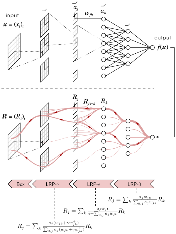
Layer-wise Relevance Propagation (LRP) is a method that identifies important pixels by running a backward pass in the neural network. The backward pass is a conservative relevance redistribution procedure, where neurons that contribute the most to the higher-layer receive most relevance from it. The LRP procedure is shown graphically in the figure below.
- Layer-wise Relevance Propagation for Deep Neural Network Architectures
- https://github.com/gentaman/LRP
- Tutorial: Implementing Layer-Wise Relevance Propagation
- http://www.heatmapping.org/
- http://iphome.hhi.de/same
Back-propagation has been the workhorse of recent successes of deep learning
but it relies on infinitesimal effects (partial derivatives) in order to perform credit
assignment. This could become a serious issue as one considers deeper and more
non-linear functions, e.g., consider the extreme case of non-linearity where the relation between parameters and cost is actually discrete. Inspired by the biological implausibility of back-propagation, a few approaches have been proposed in the past that could play a similar credit assignment role as backprop.
In this spirit, we explore a novel approach to credit assignment in deep networks that we call target propagation.
The main idea is to compute targets rather than gradients, at each layer. Like gradients, they are propagated backwards. In a way that is related but different from previously proposed proxies for back-propagation which rely on a backwards network with symmetric weights, target propagation relies on auto-encoders at each layer.
Unlike back-propagation, it can be applied even when units exchange stochastic bits rather than real numbers.
We show that a linear correction for the imperfectness of the auto-encoders is very effective to make target propagation actually work, along with adaptive learning rates.
- TARGET PROPAGATION
- Training Language Models Using Target-Propagation
- http://www2.cs.uh.edu/~ceick/
- http://www2.cs.uh.edu/~ceick/7362/7362.html
- Difference Target Propagation
We report a learning rule for neural networks that computes how much each neuron should contribute to minimize a giving cost function via the estimation of its target value. By theoretical analysis, we show that this learning rule contains backpropagation, Hebbian learning, and additional terms. We also give a general technique for weights initialization. Our results are at least as good as those obtained with backpropagation.
- Quantized Neural Networks: Training Neural Networks with Low Precision Weights and Activations
- Gradient target propagation
- https://github.com/tiago939/target
- https://qdata.github.io/deep2Read//MoreTalksTeam/Un17/Muthu-OptmTarget.pdf
- https://arxiv.org/abs/2003.10739
- https://github.com/d-li14/DHM
- http://home.cse.ust.hk/~dlibh/
- https://cqf.io/
- https://deepai.org/publication/dynamic-hierarchical-mimicking-towards-consistent-optimization-objectives
- http://home.cse.ust.hk/~dlibh/
Capsule Networks provide a way to detect parts of objects in an image and represent spatial relationships between those parts. This means that capsule networks are able to recognize the same object in a variety of different poses even if they have not seen that pose in training data.
- https://www.edureka.co/blog/capsule-networks/
- https://cezannec.github.io/Capsule_Networks/
- https://jhui.github.io/2017/11/03/Dynamic-Routing-Between-Capsules/
- Awesome Capsule Networks
- Capsule Networks Explained
- Dynamic Routing Between Capsules
- http://people.missouristate.edu/RandallSexton/sabp.pdf
- Neuronal Dynamics: From single neurons to networks and models of cognition
In contrast to known randomized learning algorithms for single layer feed-forward neural networks (e.g., random vector functional-link networks), Stochastic Configuration Networks (SCNs) randomly assign the input weights and biases of the hidden nodes in the light of a supervisory mechanism, while the output weights are analytically evaluated in a constructive or selective manner.
Current experimental results indicate that SCNs outperform other randomized neural networks in terms of required human intervention, selection of the scope of random parameters, and fast learning and generalization. `Deep stochastic configuration networks (DeepSCNs)' have been mathematically proved as universal approximators for continous nonlinear functions defined over compact sets. They can be constructed efficiently (much faster than other deep neural networks) and share many great features, such as learning representation and consistency property between learning and generalization.
This website collect some introductory material on DeepSCNs, most notably a brief selection of publications and some software to get started.
From the analytical perspective, the ad hoc nature of deep learning renders its success at the mercy of trial-and-errors.
To rectify this problem, we advocate a methodic learning paradigm, MIND-Net, which is computationally efficient in training the networks and yet mathematically feasible to analyze.
MIND-Net hinges upon the use of an effective optimization metric, called Discriminant Information (DI).
It will be used as a surrogate of the popular metrics such as 0-1 loss or prediction accuracy. Mathematically, DI is equivalent or closely related to Gauss’ LSE, Fisher’s FDR, and Shannon’s Mutual Information.
We shall explain why is that higher DI means higher linear separability, i.e. higher DI means that the data are more discriminable. In fact, it can be shown that, both theoretically and empirically, a high DI score usually implies a high prediction accuracy.
- https://datasciencephd.eu/
- https://ieeexplore.ieee.org/document/8682208
- https://www.researchgate.net/scientific-contributions/9628663_Sun-Yuan_Kung
- https://dblp.uni-trier.de/pers/hd/k/Kung:Sun=Yuan
- http://www.zhejianglab.com/mien/active_info/75.html
- https://ee.princeton.edu/people/sun-yuan-kung
- https://ieeexplore.ieee.org/author/37273489000
- Scalable Kernel Learning via the Discriminant Information
- METHODICAL DESIGN AND TRIMMING OF DEEP LEARNING NETWORKS: ENHANCING EXTERNAL BP LEARNING WITH INTERNAL OMNIPRESENT-SUPERVISION TRAINING PARADIGM