It is about how to accelerate the training and inference of deep learning(generally machine learning) except numerical optimization methods including the following topics:
- compiler optimization for computation intensive programs;
- system architecture design for computation intensive programs;
- network model compression.

- Network Compression and Acceleration
- Resource on ML Sys
- System for Deep Learning
- Compilers for Deep Learning
- Parallel Programming
- Numerical algorithms for high-performance computational science
- Deep Model Compression
- Fixed-point Arithmetic and Approximate Computing
- Huffman Encoding
- Knowledge Distillation
- Parameter Pruning and Sharing
- Quantization and Fixed-point Arithmetic
- Low Bit Neural Network
- Transferred/Compact Convolutional Filters
- Tensor Methods
- Compressing Recurrent Neural Network
- Compressing GANs
- Compressed Transformer
- Hashing-accelerated neural networks
- Distributed Training
- Products and Packages
- Edge Computation
- Inference
- Tool kits
| The World of Neural Network Acceleration |
|---|
| Choice of Algorithm |
| Parallelism |
| Distributed Computing |
| Hardware Architectures |
- Trax — your path to advanced deep learning
- THE 5TH ANNUAL SCALEDML CONFERENCE
- https://www.atlaswang.com/
- https://faculty.ucmerced.edu/mcarreira-perpinan/research/MCCO.html
- https://github.com/1duo/awesome-ai-infrastructures
- https://duvenaud.github.io/learning-to-search/
- http://www.eecs.harvard.edu/htk/publications/
- http://www.eecs.harvard.edu/htk/courses/
- FairNAS: Rethinking Evaluation Fairness of Weight Sharing Neural Architecture Search
- VISUAL COMPUTING SYSTEMS
- Tutorial on Hardware Accelerators for Deep Neural Networks
- Survey and Benchmarking of Machine Learning Accelerators
- https://zhuanlan.zhihu.com/jackwish
- https://machinethink.net/blog/compressing-deep-neural-nets/
- Rethinking Deep Learning: Architectures and Algorithms
- https://girishvarma.in/teaching/efficient-cnns/
- https://github.com/ChanChiChoi/awesome-model-compression
- https://github.com/fengbintu/Neural-Networks-on-Silicon
- https://vast.cs.ucla.edu/
- Blade Benchmark Suite(BBS)简介
- https://web.northeastern.edu/yanzhiwang/research/
- http://shivaram.org/#teaching
- https://neuralmagic.com/blog/
- https://github.com/PredictiveModelingMachineLearningLab/MA598
- https://c3dti.ai/
- https://statistics.wharton.upenn.edu/profile/dobriban/
- https://ml-retrospectives.github.io/
- https://data.berkeley.edu/
- https://github.com/mcanini/SysML-reading-list
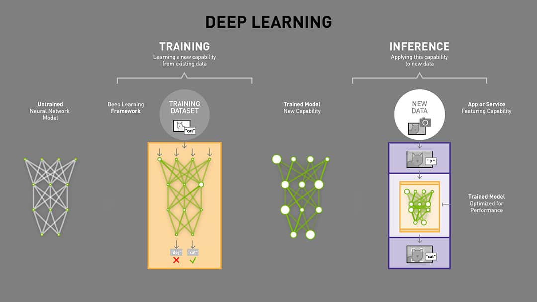
The parameters of deep neural networks are tremendous. And deep learning is matrix-computation intensive.
Specific hardware such as GPU or TPU is used to speed up the computation of deep learning in training or inference.
The optimization methods are used to train the deep neural network.
To boost the training of deep learning,
we would like to design faster optimization methods such as ADAM and delicate architectures of neural network such as ResNet.
After training, the parameters of the deep neural network are fixed and used for inference,
we would do much matrix multiplication via the saved fixed parameters of deep neural network.
From What’s the Difference Between Deep Learning Training and Inference?
| Evolution of Model Compression and Acceleration |
|---|
| Computer Architecture: TPUs, GPUs |
| Compilers: TVM |
| Model Re-design: EfficientNet |
| Re-parameterization: Pruning |
| Transfer Learning |
When the computation resource is limited such as embedded or mobile system, can we deploy deep learning models? Definitely yes.
- Awesome model compression and acceleration
- Acceleration and Model Compression by Handong
- Accelerating Deep Learning Inference via Freezing
- 模型压缩之deep compression
- 论文笔记《A Survey of Model Compression and Acceleration for Deep Neural Networks》
- https://zhuanlan.zhihu.com/p/67508423
- Network Speed and Compression
- Model Compression and Acceleration
- Deep Compression: Compressing Deep Neural Networks with Pruning, Trained Quantization and Huffman Coding
- Deep Gradient Compression: Reducing the Communication Bandwidth for Distributed Training
- AutoML 的十大开源库
- TensorFlow模型压缩和Inference加速
- https://zhuanlan.zhihu.com/DNN-on-Chip
- https://github.com/BlueWinters/research
- Reference workloads for modern deep learning methods
- How to Train for and Run Machine Learning Models on Edge Devices
- http://mvapich.cse.ohio-state.edu/
- http://people.eecs.berkeley.edu/~reddy/
- Neural Network Calibration
- http://www.sysml.cc/
- https://mlperf.org/
- https://sosp19.rcs.uwaterloo.ca/program.html
- http://learningsys.org/sosp19/schedule.html
- https://cs.stanford.edu/people/zhihao/
- Workshop on AI Systems
- Systems for ML
- Workshop on ML for Systems at NeurIPS 2019
- http://learningsys.org/nips18/
- http://learningsys.org/sosp17/
- https://sites.google.com/site/mlsys2016/
- Workshop on Systems for ML and Open Source Software at NeurIPS 2018
- Computer Systems Colloquium (EE380) Schedule
- ML Benchmarking Tutorial
- The ACM Joint European Software Engineering Conference and Symposium on the Foundations of Software Engineering (ESEC/FSE)
- The fastest path to machine learning integration
- https://www.sigarch.org/call-participation/ml-benchmarking-tutorial/
- DNNBuilder: an Automated Tool for Building High-Performance DNN Hardware Accelerators for FPGAs
- ISCA 2016 in Seoul
- Acceleration of Deep Learning for Cloud and Edge Computing@UCLA
- Hot Chips: A Symposium on High Performance Chips
- https://paco-cpu.github.io/paco-cpu/
- Programmable Inference Accelerator
- Fair and useful benchmarks for measuring training and inference performance of ML hardware, software, and services.
- https://dlonsc19.github.io/
- https://www.nextplatform.com/
- https://iq.opengenus.org/neural-processing-unit-npu/
- https://www.csail.mit.edu/event/domain-specific-accelerators
- https://www.alphaics.ai/
- http://www.cambricon.com/
- https://www.sigarch.org/
- https://www.xilinx.com/
- https://wavecomp.ai/
- https://www.graphcore.ai/
- https://www.wikiwand.com/en/Hardware_acceleration
- https://en.wikichip.org/wiki/WikiChip
- https://patents.google.com/patent/US8655815B2/en
- https://www.intel.ai/blog/
- https://www.arm.com/solutions/artificial-intelligence
- https://mlperf.org/index.html#companies
- Accelerating Deep Learning with Memcomputing
- http://maxpumperla.com/
- http://accelergy.mit.edu/
- https://eng.uber.com/sbnet-sparse-block-networks-convolutional-neural-networks/
- Modern Numerical Computing
- Papers Reading List of Embedded Neural Network
- Deep Compression and EIE
- Programmable Hardware Accelerators (Winter 2019)
- Hardware Accelerators for Training Deep Neural Networks
- Illinois Microarchitecture Project using Algorithms and Compiler Technology
- Deep Learning for Computer Architects
- System for Machine Learning @.washington.edu/
- Hanlab: ACCELERATED DEEP LEARNING COMPUTING Hardware, AI and Neural-nets
- Bingsheng He's publication on GPU
- Architecture Lab for Creative High-performance Energy-efficient Machines
- HIGH PERFORMANCE POWER EFFICIENT NEURAL NETWORK IMPLEMENTATIONS ON EMBEDDED DEVICES
- https://eiclab.net/
- https://parsa.epfl.ch/~falsafi/
- swDNN: A Library for Accelerating Deep Learning Applications on Sunway TaihuLight Supercomputer
- High Performance Distributed Computing (HPDC
- https://readingxtra.github.io/
- https://nextcenter.org/
- http://yanjoy.win/
- https://dlonsc19.github.io/
- http://hibd.cse.ohio-state.edu/
- http://www.federated-ml.org/
- https://dai.lids.mit.edu/research/publications/
- https://aiforgood.itu.int/
- https://www.linayao.com/publications/
- https://www.deepstack.ai/
- https://pvs.ifi.uni-heidelberg.de/home
Over the past few years, deep learning has become an important technique to successfully solve problems in many different fields, such as vision, NLP, robotics. An important ingredient that is driving this success is the development of deep learning systems that efficiently support the task of learning and inference of complicated models using many devices and possibly using distributed resources. The study of how to build and optimize these deep learning systems is now an active area of research and commercialization.
Matrix computation dense application like deep neural network would take the advantages of specific architecture design.
Thus it is really close to high performance computational science when solving some computation dense problems.

- BENCHMARKING DEEP LEARNING SYSTEMS
- Facebook AI Performance Evaluation Platform
- Hardware Accelerators for Machine Learning (CS 217) Stanford University, Fall 2018
- CSCE 790/590: Machine Learning Systems
- DeepDream: Accelerating Deep Learning With Hardware
- http://ece-research.unm.edu/jimp/codesign/
- http://learningsys.org/sosp19/
- https://determined.ai/
- https://web.stanford.edu/~rezab/
Parallel Architectures for Parallel Processing as co-design is a subfield of system for machine learning.
- https://vistalab-technion.github.io/cs236605/lectures/lecture_8/
- https://vistalab-technion.github.io/cs236605/lectures/lecture_9/
- https://vistalab-technion.github.io/cs236605/lectures/lecture_10/
- https://iq.opengenus.org/gpu-vs-tpu-vs-fpga/
- Introduction to Parallel Computing Author: Blaise Barney, Lawrence Livermore National Laboratory
- Parallel Architectures for Artificial Neural Networks: Paradigms and Implementations N. Sundararajan, P. Saratchandran
- Parallel Computer Architecture and Programming (CMU 15-418/618)
- https://twimlcon.com/
- Accelerating Deep Learning with a Parallel Mechanism Using CPU + MIC
- Papers on Big Data Meets New Hardware
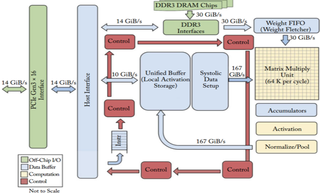
This GPU architecture works well on applications with massive parallelism, such as matrix multiplication in a neural network. Actually, you would see order of magnitude higher throughput than CPU on typical training workload for deep learning. This is why the GPU is the most popular processor architecture used in deep learning at time of writing.
But, the GPU is still a general purpose processor that has to support millions of different applications and software. This leads back to our fundamental problem, the von Neumann bottleneck. For every single calculation in the thousands of ALUs, GPU need to access registers or shared memory to read and store the intermediate calculation results. Because the GPU performs more parallel calculations on its thousands of ALUs, it also spends proportionally more energy accessing memory and also increases footprint of GPU for complex wiring.

TPUs can't run word processors, control rocket engines, or execute bank transactions, but they can handle the massive multiplications and additions for neural networks, at blazingly fast speeds while consuming much less power and inside a smaller physical footprint.
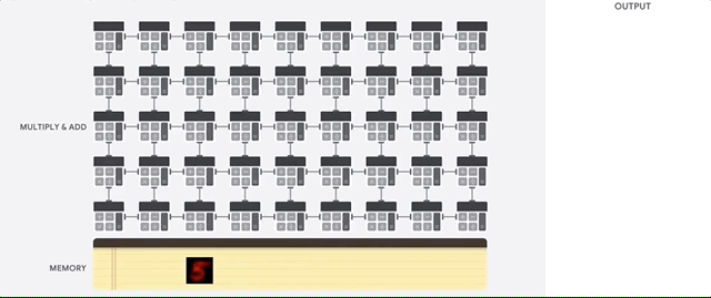
The key enabler is a major reduction of the von Neumann bottleneck. Because the primary task for this processor is matrix processing, hardware designer of the TPU knew every calculation step to perform that operation. So they were able to place thousands of multipliers and adders and connect them to each other directly to form a large physical matrix of those operators. This is called systolic array architecture.


- In-Datacenter Performance Analysis of a Tensor Processing Unit
- https://www.mlq.ai/tpu-machine-learning/
- EfficientNet-EdgeTPU: Creating Accelerator-Optimized Neural Networks with AutoML
- An in-depth look at Google’s first Tensor Processing Unit (TPU)
- A Domain-Specific Architecture for Deep Neural Networks
A neural processing unit (NPU) is a microprocessor that specializes in the acceleration of machine learning algorithms, typically by operating on predictive models such as artificial neural networks (ANNs) or random forests (RFs). It is, also, known as neural processor.
NPU are required for the following purpose:
- Accelerate the computation of Machine Learning tasks by several folds (nearly 10K times) as compared to GPUs
- Consume low power and improve resource utilization for Machine Learning tasks as compared to GPUs and CPUs
- https://aiotworkshop.github.io/2020/program.html
- https://www.incose.org/
- Compilers by SOE-YCSCS1 STANFORD SCHOOL OF ENGINEERING
- EIE: Efficient Inference Engine on Compressed Deep Neural Network
- A modern compiler infrastructure for deep learning systems with adjoint code generation in a domain-specific IR
- https://ai-techsystems.com/dnn-compiler/
The LLVM Project is a collection of modular and reusable compiler and toolchain technologies. Despite its name, LLVM has little to do with traditional virtual machines. The name "LLVM" itself is not an acronym; it is the full name of the project.
The Multi-Level Intermediate Representation (MLIR) is intended for easy expression and optimization of computations involving deep loop nests and dense matrices of high dimensionality.
It is thus well-suited to deep learning computations in particular.
Yet it is general enough to also represent arbitrary sequential computation.
The representation allows high-level optimization and parallelization for a wide range of parallel architectures including those with deep memory hierarchies --- general-purpose multicores, GPUs, and specialized neural network accelerators.
- https://github.com/tensorflow/mlir
- https://llvm.org/devmtg/2019-04/slides/Keynote-ShpeismanLattner-MLIR.pdf
IREE (Intermediate Representation Execution Environment1) is an MLIR-based end-to-end compiler and runtime that lowers Machine Learning (ML) models to a unified IR that scales up to meet the needs of the datacenter and down to satisfy the constraints and special considerations of mobile and edge deployments.
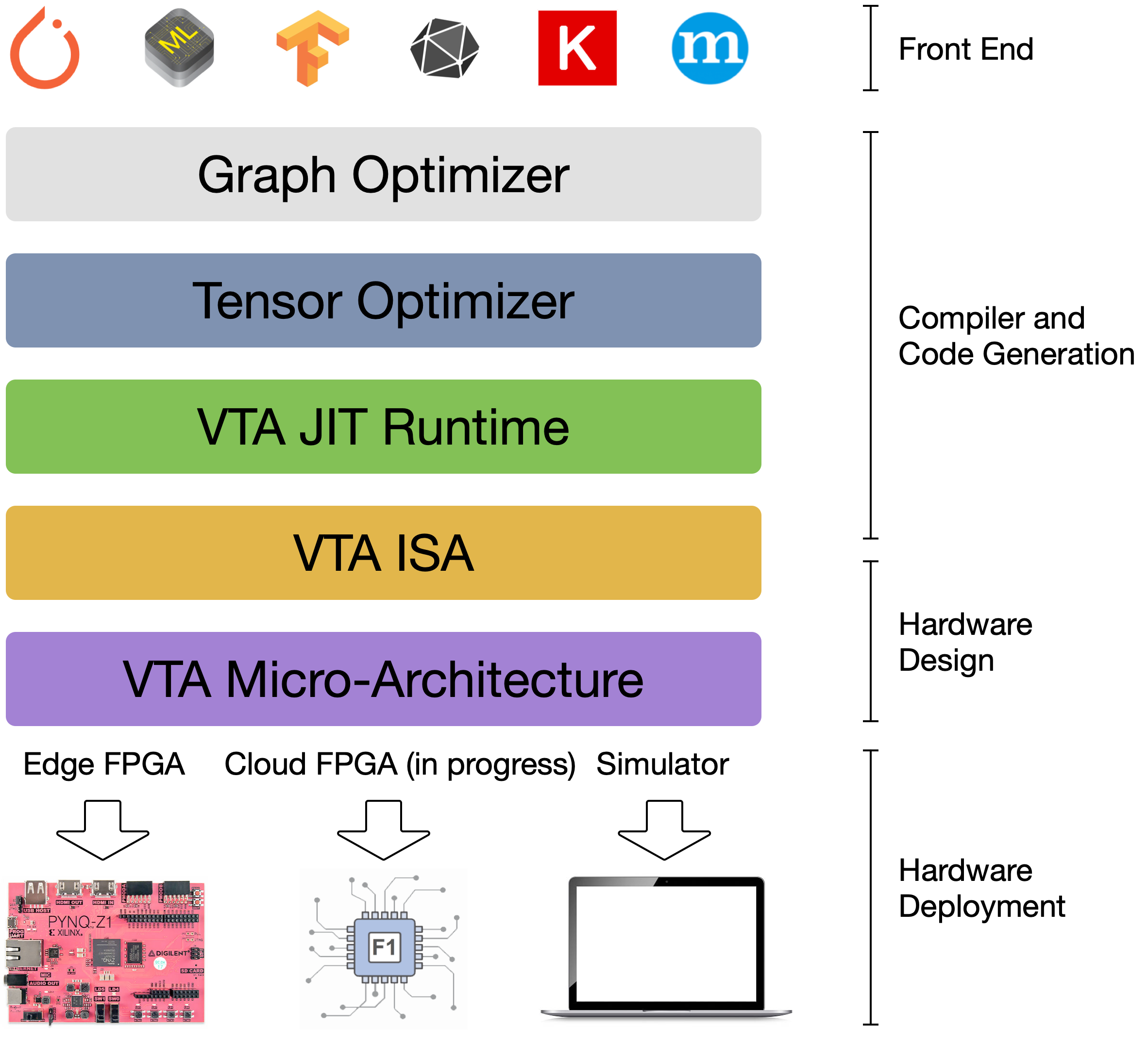
TVM is an open deep learning compiler stack for CPUs, GPUs, and specialized accelerators. It aims to close the gap between the productivity-focused deep learning frameworks, and the performance- or efficiency-oriented hardware backends. TVM provides the following main features:
Compilation of deep learning models in Keras, MXNet, PyTorch, Tensorflow, CoreML, DarkNet into minimum deployable modules on diverse hardware backends. Infrastructure to automatic generate and optimize tensor operators on more backend with better performance.
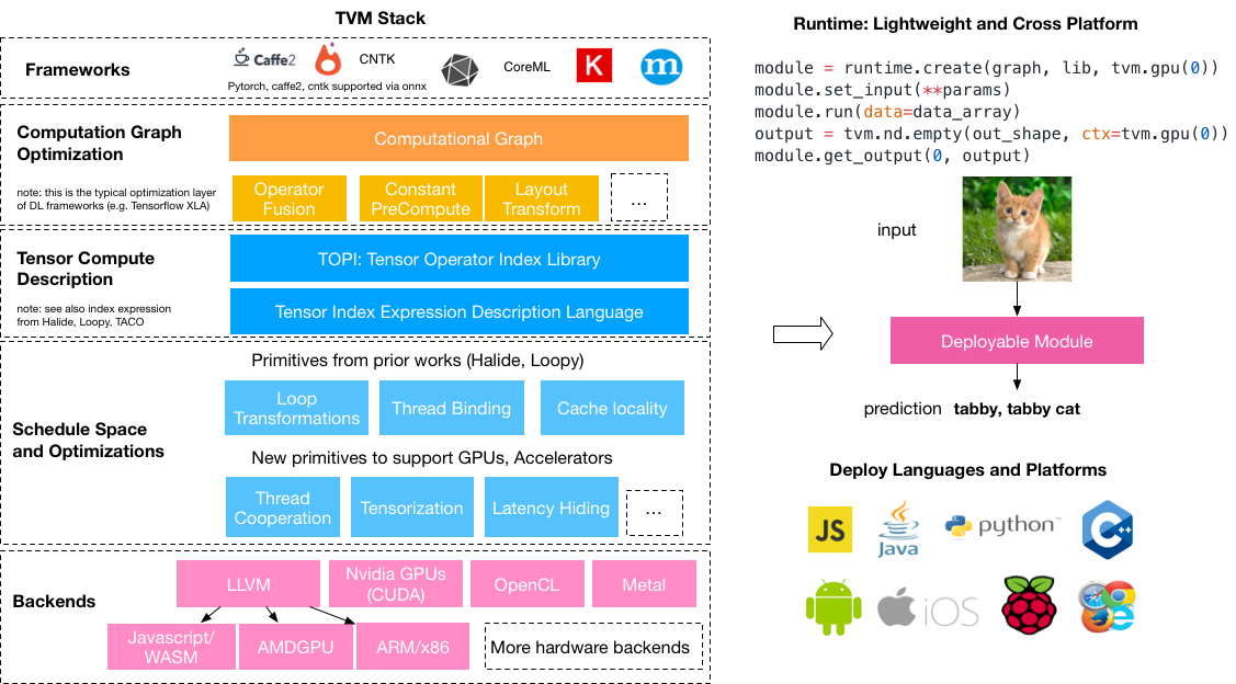
The Versatile Tensor Accelerator (VTA) is an extension of the TVM framework designed to advance deep learning and hardware innovation. VTA is a programmable accelerator that exposes a RISC-like programming abstraction to describe compute and memory operations at the tensor level. We designed VTA to expose the most salient and common characteristics of mainstream deep learning accelerators, such as tensor operations, DMA load/stores, and explicit compute/memory arbitration.
- https://sampl.cs.washington.edu/
- https://homes.cs.washington.edu/~haichen/
- https://tqchen.com/
- https://www.cs.washington.edu/people/faculty/arvind
- TVM: End to End Deep Learning Compiler Stack
- TVM and Deep Learning Compiler Conference
- VTA Deep Learning Accelerator
- https://sampl.cs.washington.edu/
- https://docs.tvm.ai/vta/index.html
- 如何利用TVM快速实现超越Numpy(MKL)的GEMM蓝色
- 使用TVM支持TFLite(下)
We present DLVM, a design and implementation of a compiler infrastructure with a linear algebra intermediate representation, algorithmic differentiation by adjoint code generation, domain-specific optimizations, and a code generator targeting GPU via LLVM.
- DLVM: A MODERN COMPILER INFRASTRUCTURE FOR DEEP LEARNING SYSTEMS
- https://github.com/dlvm-team
- https://github.com/Jittor/jittor
- http://dlvm.org/
- http://dowobeha.github.io/papers/autodiff17.pdf
- http://dowobeha.github.io/
- https://roshandathathri.github.io/
- https://www.clsp.jhu.edu/workshops/19-workshop/
With its updated version of Autograd, JAX can automatically differentiate native Python and NumPy functions. It can differentiate through loops, branches, recursion, and closures, and it can take derivatives of derivatives of derivatives. It supports reverse-mode differentiation (a.k.a. backpropagation) via grad as well as forward-mode differentiation, and the two can be composed arbitrarily to any order.
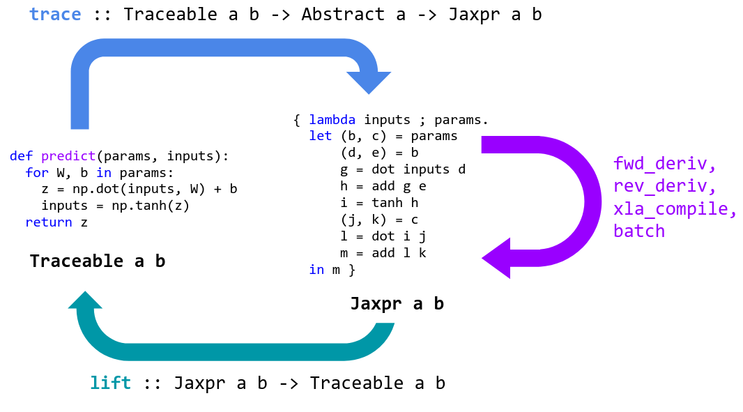
The XLA compilation framework is invoked on subgraphs of TensorFlow computations. The framework requires all tensor shapes to be fixed, so compiled code is specialized to concrete shapes. This means, for example, that the compiler may be invoked multiple times for the same subgraph if it is executed on batches of different sizes.
- https://www.tensorflow.org/versions/master/experimental/xla/
- https://developers.googleblog.com/2017/03/xla-tensorflow-compiled.html
- https://www.tensorflow.org/xla/overview
- https://autodiff-workshop.github.io/slides/JeffDean.pdf
- XLA: The TensorFlow compiler framework
Glow is a machine learning compiler and execution engine for hardware accelerators.
It is designed to be used as a backend for high-level machine learning frameworks.
The compiler is designed to allow state of the art compiler optimizations and code generation of neural network graphs.
This library is in active development.
- https://arxiv.org/pdf/1805.00907.pdf
- https://ai.facebook.com/tools/glow/
- https://github.com/pytorch/glow
nGraph is an end to end deep learning compiler for inference and training with extensive framework and hardware support.

CHET is a domain-specific optimizing compiler designed to make the task of programming FHE applications easier. Motivated by the need to perform neural network inference on encrypted medical and financial data, CHET supports a domain-specific language for specifying tensor circuits. It automates many of the laborious and error prone tasks of encoding such circuits homomorphically, including encryption parameter selection to guarantee security and accuracy of the computation, determining efficient tensor layouts, and performing scheme-specific optimizations.
- https://roshandathathri.github.io/publication/2019-pldi
- CHET: An Optimizing Compiler for Fully-Homomorphic Neural-Network Inferencing
- https://www.cs.utexas.edu/~pingali/
- https://roshandathathri.github.io/
- https://iss.oden.utexas.edu/
NNFusion is a flexible and efficient DNN compiler that can generate high-performance executables from a DNN model description (e.g., TensorFlow frozen models and ONNX format).
- Rammer: Enabling Holistic Deep Learning Compiler Optimizations with rTasks
- https://github.com/microsoft/nnfusion
- https://www.opensourceagenda.com/projects/nnfusion
DLR is a compact, common runtime for deep learning models and decision tree models compiled by AWS SageMaker Neo, TVM, or Treelite. DLR uses the TVM runtime, Treelite runtime, NVIDIA TensorRT™, and can include other hardware-specific runtimes. DLR provides unified Python/C++ APIs for loading and running compiled models on various devices. DLR currently supports platforms from Intel, NVIDIA, and ARM, with support for Xilinx, Cadence, and Qualcomm coming soon.
- https://github.com/neo-ai/neo-ai-dlr
- https://github.com/dmlc/treelite
- http://treelite.io/
- https://aws.amazon.com/cn/sagemaker/neo/
- https://www.openmp.org/
- https://www.open-mpi.org/
- https://www.khronos.org/opencl/
- https://developer.nvidia.com/opencl
- https://opencl.org/
Cilk aims to make parallel programming a simple extension of ordinary serial programming. Other concurrency platforms, such as Intel’s Threading Building Blocks (TBB) and OpenMP, share similar goals of making parallel programming easier. But Cilk sets itself apart from other concurrency platforms through its simple design and implementation and its powerful suite of provably effective tools. These properties make Cilk well suited as a platform for next-generation multicore research. Tapir enables effective compiler optimization of parallel programs with only minor changes to existing compiler analyses and code transformations. Tapir uses the serial-projection property to order logically parallel fine-grained tasks in the program's control-flow graph. This ordered representation of parallel tasks allows the compiler to optimize parallel codes effectively with only minor modifications.
The aim of Triton is to provide an open-source environment to write fast code at higher productivity than CUDA, but also with higher flexibility than other existing DSLs.
- Triton: An Intermediate Language and Compiler for Tiled Neural Network Computations
- https://github.com/ptillet/triton
- https://pldi19.sigplan.org/details/mapl-2019-papers/1/Triton-An-Intermediate-Language-and-Compiler-for-Tiled-Neural-Network-Computations
- http://www.federated-ml.org/tutorials/globecom2020/part4.pdf
TASO optimizes the computation graphs of DNN models using automatically generated and verified graph transformations. For an arbitrary DNN model, TASO uses the auto-generated graph transformations to build a large search space of potential computation graphs that are equivalent to the original DNN model. TASO employs a cost-based search algorithm to explore the space, and automatically discovers highly optimized computation graphs.
- https://cs.stanford.edu/people/zhihao/
- https://github.com/jiazhihao/TASO
- http://theory.stanford.edu/~aiken/
Jittor is a high-performance deep learning framework based on JIT compiling and meta-operators. The whole framework and meta-operators are compiled just-in-time. A powerful op compiler and tuner are integrated into Jittor. It allowed us to generate high-performance code with specialized for your model. Jittor also contains a wealth of high-performance model libraries, including: image recognition, detection, segmentation, generation, differentiable rendering, geometric learning, reinforcement learning, etc.。
Halide is a programming language designed to make it easier to write high-performance image and array processing code on modern machines.
Halide is a language for fast, portable computation on images and tensors
Taichi (太极) is a programming language designed for high-performance computer graphics. It is deeply embedded in Python, and its just-in-time compiler offloads compute-intensive tasks to multi-core CPUs and massively parallel GPUs.
Taichi Lang is an open-source, imperative, parallel programming language for high-performance numerical computation. It is embedded in Python and uses just-in-time (JIT) compiler frameworks, for example LLVM, to offload the compute-intensive Python code to the native GPU or CPU instructions.
Several key themes emerged across multiple talks in Royal Society Discussion Meeting, all in the context of today’s high performance computing landscape in which processor clock speeds have stagnated (with the end of Moore’s law) and exascale machine are just two or three years away.
- An important way of accelerating computations is through the use of
low precision floating-point arithmetic—in particular by exploiting a hierarchy of precisions. - We must exploit
low rank matrix structurewhere it exists, for example in hierarchical (H-matrix) form, combining it with randomized approximations. - Minimizing
data movement (communication)is crucial, because of its increasing costs relative to the costs of floating-point arithmetic. Co-design(the collaborative and concurrent development of hardware, software, and numerical algorithms, with knowledge of applications) is increasingly important for numerical computing.
For more on high performance computation on GPU see https://hgpu.org/.
- https://hgpu.org/
- Numerical Algorithms for High-Performance Computational Science: Highlights of the Meeting
- Numerical algorithms for high-performance computational science
- Reflections on the Royal Society’s “Numerical Algorithms for High-performance Computational Science” Discussion Meeting
- Overview of Microsoft HPC Pack 2016
- Document Library: High Performance Computing Fabrics
- MVAPICH: MPI over InfiniBand, Omni-Path, Ethernet/iWARP, and RoCE
- https://researchcomputing.lehigh.edu/
- https://library.columbia.edu/libraries/dsc/hpc.html
- Open MPI: Open Source High Performance Computing
- https://ltsnews.lehigh.edu/node/115
- NumFOCUS
- http://www.mit.edu/~kepner/D4M/
- CSCS-ICS-DADSi Summer School: Accelerating Data Science with HPC, September 4 – 6, 2017
- MS&E 317: Algorithms for Modern Data Models: Spring 2014, Stanford University
- Distributed Machine Learning and Matrix Computations: A NIPS 2014 Workshop
- Large Scale Matrix Analysis and Inference: A NIPS 2013 Workshop
- Breakthrough! Faster Matrix Multiply
- Performance Engineering of Software Systems
- https://zhuanlan.zhihu.com/p/94653447
Why GEMM is at the heart of deep learning

Matrix-vector multiplication is a special matrix multiplication:
- https://people.csail.mit.edu/rrw/
- Matrix-Vector Multiplication in Sub-Quadratic Time (Some Preprocessing Required)
- The Mailman algorithm for matrix vector multiplication
- Matrix-vector multiplication using the FFT
- On fast matrix-vector multiplication with a Hankel matrix in multiprecision arithmetics
- Optimizing Large Matrix-Vector Multiplications
- Faster Matrix vector multiplication ON GeForce
- Fast Implementation of General Matrix-Vector Multiplication (GEMV) on Kepler GPUs
- FAST ALGORITHMS TO COMPUTE MATRIX-VECTOR PRODUCTS FOR PASCAL MATRICES
- Fast algorithms to compute matrix-vector products for Toeplitz and Hankel matrices
- Fast High Dimensional Vector Multiplication Face Recognition
- Faster Online Matrix-Vector Multiplication
- A fast matrix–vector multiplication method for solving the radiosity equation
- Computational Science and Engineering Spring 2015 syllabus
Generations of students have learned that the product matrix chain multiplication problem.
A special case is when
- The World’s Most Fundamental Matrix Equation
- Computation of Matrix Chain Products, PART I, PART II
- CS3343/3341 Analysis of Algorithms Matrix-chain Multiplications
- rosettacode: Matrix chain multiplication
- http://www.columbia.edu/~cs2035/courses/csor4231.F11/matrix-chain.pdf
- https://www.geeksforgeeks.org/matrix-chain-multiplication-dp-8/
- https://www.geeksforgeeks.org/matrix-chain-multiplication-a-on2-solution/
- https://home.cse.ust.hk/~dekai/271/notes/L12/L12.pdf
If the computation speed of matrix operation is boosted, the inference of deep learning model is accelerated.
Matrix multiplication
which is esentially product-sum.
for (int m = 0; m < M; m++) {
  for (int n = 0; n < N; n++) {
    C[m][n] = 0;
    for (int k = 0; k < K; k++) {
      C[m][n] += A[m][k] * B[k][n];
    }
  }
}

It needs
The picture below visualizes the computation of a single element in the result matrix

Our program is memory bound, which means that the multipliers are not active most of the time because they are waiting for memory.
- Anatomy of High-Performance Matrix Multiplication
- Geometry and the complexity of matrix multiplication
- High-Performance Matrix Multiplication
- Fast Matrix Multiplication @mathoverflow
- Powers of Tensors and Fast Matrix Multiplication
- https://www.kkhaydarov.com/matrix-multiplication-algorithms/
- BLISlab: A Sandbox for Optimizing GEMM
- MAGMA: Matrix Algebra for GPU and Multicore Architectures
- http://apfel.mathematik.uni-ulm.de/~lehn/sghpc/gemm/
- 通用矩阵乘和卷积优化
- Fast Matrix Multiplication Algorithms
- Anatomy of high-performance matrix multiplication
- The Indirect Convolution Algorithm
- https://github.com/flame/how-to-optimize-gemm/wiki
- https://en.wikipedia.org/wiki/Matrix_multiplication#Complexity
- Matrix multiplication via arithmetic progressions
- Fast sparse matrix multiplication
- Part I: Performance of Matrix multiplication in Python, Java and C++
- Part III: Matrix multiplication on multiple cores in Python, Java and C++
- https://github.com/MartinThoma/matrix-multiplication
- http://jianyuhuang.com/
- SPATIAL: A high-level language for programming accelerators
- https://github.com/OAID/Tengine
- Performance of Classic Matrix Multiplication Algorithm on Intel® Xeon Phi™ Processor System
- Low-precision matrix multiplication
It is based on block-multiplication. It is required that
The matrice are rearranged as blocks: $$ \mathbf{A} = \begin{bmatrix} \mathbf{A}{1,1} & \mathbf{A}{1,2} \ \mathbf{A}{2,1} & \mathbf{A}{2,2} \end{bmatrix}, \mathbf{B} = \begin{bmatrix} \mathbf{B}{1,1} & \mathbf{B}{1,2} \ \mathbf{B}{2,1} & \mathbf{B}{2,2} \end{bmatrix},\ \mathbf{C} = \begin{bmatrix} \mathbf{C}{1,1} & \mathbf{C}{1,2} \ \mathbf{C}{2,1} & \mathbf{C}{2,2} \end{bmatrix} = \begin{bmatrix} \mathbf{A}{1,1}\mathbf{B}{1,1} & \mathbf{A}{1,2}\mathbf{B}{1,2} \ \mathbf{A}{2,1}\mathbf{B}{2,1} & \mathbf{A}{2,2}\mathbf{B}{2,2} \end{bmatrix}. $$
Submatrix(blocks) multiplication is performed in the following way: $$ \mathbf{M}{1} =\left(\mathbf{A}{1,1}+\mathbf{A}{2,2}\right)\left(\mathbf{B}{1,1}+\mathbf{B}{2,2}\right) \ \mathbf{M}{2} =\left(\mathbf{A}{2,1}+\mathbf{A}{2,2}\right) \mathbf{B}{1,1} \ \mathbf{M}{3} =\mathbf{A}{1,1}\left(\mathbf{B}{1,2}-\mathbf{B}{2,2}\right) \ \mathbf{M}{4} =\mathbf{A}{1,2}\left(\mathbf{B}{2,1}-\mathbf{B}{1,1}\right) \ \mathbf{M}{5} =\left(\mathbf{A}{1,1}+\mathbf{A}{1,2}\right) \mathbf{B}{2,2} \ \mathbf{M}{6} =\left(\mathbf{A}{2,1}-\mathbf{A}{1,1}\right)\left(\mathbf{B}{1,1}+\mathbf{B}{1,2}\right) \ \mathbf{M}{7} =\left(\mathbf{A}{1,2}-\mathbf{A}{2,2}\right)\left(\mathbf{B}{2,1}+\mathbf{B}_{2,2}\right) $$
And then $$ \mathbf{C}{1,1} =\mathbf{M}{1}+\mathbf{M}{4}-\mathbf{M}{5}+\mathbf{M}{7} \ \mathbf{C}{1,2} =\mathbf{M}{3}+\mathbf{M}{5} \ \mathbf{C}{2,1} =\mathbf{M}{2}+\mathbf{M}{4} \ \mathbf{C}{2,2} =\mathbf{M}{1}-\mathbf{M}{2}+\mathbf{M}{3}+\mathbf{M}{6} $$
- Strassen’s Matrix Multiplication Algorithm | Implementation
- Part II: The Strassen algorithm in Python, Java and C++
- Using Strassen’s Algorithm to Accelerate the Solution of Linear System
- https://shivathudi.github.io/jekyll/update/2017/06/15/matr-mult.html
- http://jianyuhuang.com/papers/sc16.pdf
- Comparative Study of Strassen’s Matrix Multiplication Algorithm
- http://andrew.gibiansky.com/blog/mathematics/matrix-multiplication/
- http://jianyuhuang.com/
For matrix multiplication
The tensor corresponding to the multiplication of an
One can define in a natural way the tensor product of two tensors. In particular, for matrix multipli-
cation tensors, we obtain the following identity: for any positive integers
Consider three vector spaces
-
$U=span{x_1, \dots, x_{dim(U)}}$ , -
$V=span{y_1, \dots, y_{dim(U)}}$ , -
$W=span{z_1, \dots, z_{dim(U)}}$ .
A tensor over
We use tensors (and their low-rank decompositions) to multiply matrices faster than $O(n^3)$.
Define the matrix multiplication tensor as follows:
$$
M_{(a, b), (c, d), (e, f)}^{(n)}
=\begin{cases}
1, &\text{if
Then we can use this decomposition to re-express matrix multiplication: $$ {(AB)}{ik}=\sum{j}A_{ij}B_{jk}\ =\sum_{j}M_{(i, j), (j, k), (k, i)}^{(n)}A_{ij}B_{jk}\ = \sum_{a=1}^n\sum_{b=1}^n\sum_{c=1}^n\sum_{d=1}^n M_{(a, b), (c, d), (k, i)}^{(n)}A_{ab}B_{cd}\ = \sum_{a=1}^n\sum_{b=1}^n\sum_{c=1}^n\sum_{d=1}^n (\sum_{l=1}^{r} x_{ab}^l y_{cd}^l z_{ki}^l)A_{ab}B_{cd}\ = \sum_{l=1}^r z_{ki}^l(\sum_{a=1}^n\sum_{b=1}^n x_{ab}^l A_{ab})(\sum_{c=1}^n\sum_{d=1}^n y_{cd}^l B_{cd}) $$
- Fast Matrix Multiplication = Calculating Tensor Rank, Caltech Math 10 Presentation
- http://users.wfu.edu/ballard/pdfs/CSE17.pdf
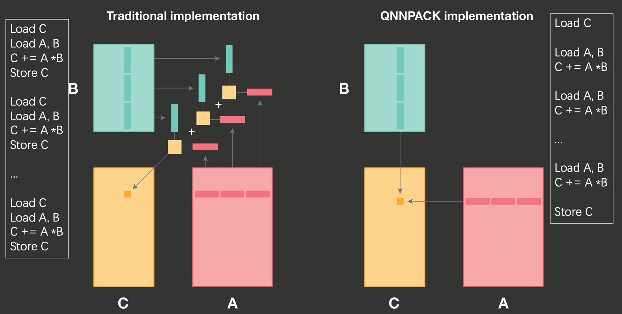
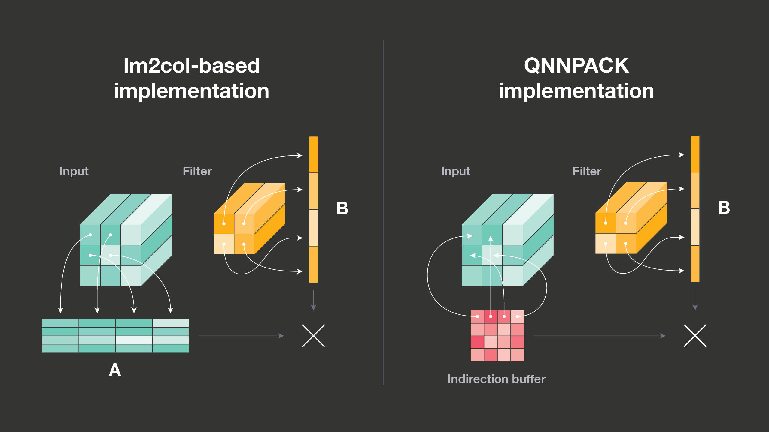
- https://jackwish.net/reveal-qnnpack-implementation.html
- Coppersmith-Winograd Algorithm
- On the Coppersmith–Winograd method
- Adaptive Winograd’s Matrix Multiplications
- https://www.wikiwand.com/en/Matrix_multiplication_algorithm
- Introduction to fast matrix multiplication
- Practical Fast Matrix Multiplication Algorithms
- Breaking the Coppersmith-Winograd barrier
- Multiplying matrices faster than Coppersmith-Winograd
- Limits on All Known (and Some Unknown) Approaches to Matrix Multiplication
- A New Fast Recursive Matrix Multiplication Algorithm
- https://cqa.institute/2015/08/07/accelerating-matrix-multiplication/
- Distinguished Lecture Series III: Avi Wigderson, “Algebraic computation”
- http://www.cs.utexas.edu/~rvdg/
- Halide: a language for fast, portable computation on images and tensors
- https://eigen.tuxfamily.org/dox/index.html
- FLAME project
- A high-level language for programming accelerators
- http://people.ece.umn.edu/users/parhi/
- https://www.cs.utexas.edu/~flame/web/publications.html
- PLAPACK: Parallel Linear Algebra Package
- https://spatial-lang.readthedocs.io/en/latest/
- Matrix Computations and Optimization in Apache Spark
- Cusp is a library for sparse linear algebra and graph computations based on Thrust.
- The Hierarchical Computations on Manycore Architectures (HiCMA) library aims to redesign existing dense linear algebra libraries to exploit the data sparsity of the matrix operator.
- A generalized multidimensional matrix multiplication
- https://dspace.mit.edu/handle/1721.1/85943
- BLIS Retreat 2017
Fast linear transforms are ubiquitous in machine learning, including the discrete Fourier transform, discrete cosine transform,
and other structured transformations such as convolutions.
All of these transforms can be represented by dense matrix-vector multiplication, yet each has a specialized and highly efficient (subquadratic) algorithm.
We ask to what extent hand-crafting these algorithms and implementations is necessary, what structural priors they encode,
and how much knowledge is required to automatically learn a fast algorithm for a provided structured transform.
Motivated by a characterization of fast matrix-vector multiplication as products of sparse matrices,
we introduce a parameterization of divide-and-conquer methods that is capable of representing a large class of transforms.
This generic formulation can automatically learn an efficient algorithm for many important transforms;
for example, it recovers the
- Learning Fast Algorithms for Linear Transforms Using Butterfly Factorizations
- Learning Fast Algorithms for Linear Transforms Using Butterfly Factorizations
- Butterflies Are All You Need: A Universal Building Block for Structured Linear Maps
- https://github.com/stanford-futuredata/Willump
- A Two Pronged Progress in Structured Dense Matrix Multiplication
All numerical gradient-based optimization methods benefits from faster computation of gradients specially backprop.
Many algorithms in machine learning, computer vision, physical simulation, and other fields require the calculation of
gradients and other derivatives. Manual derivation of gradients can be time consuming and error-prone.Automatic Differentiation (AD)is a technology for automatically augmenting computer programs, including arbitrarily complex simulations, with statements for the computation of derivatives, also known as sensitivities. Automatic differentiation comprises a set of techniques to calculate the derivative of a numerical computation expressed as a computer program. These techniques are commonly used in atmospheric sciences and computational fluid dynamics, and have more recently also been adopted by machine learning researchers. Practitioners across many fields have built a wide set of automatic differentiation tools, using different programming languages, computational primitives and intermediate compiler representations. Each of these choices comes with positive and negative trade-offs, in terms of their usability, flexibility and performance in specific domains.
In the ideal case, automatically generated derivatives should be competitive with manually generated ones and run at near-peak performance on modern hardware, but the most expressive systems for autodiff which can handle arbitrary, Turing-complete programs, are unsuited for performance-critical applications, such as large-scale machine learning or physical simulation. Alternatively, the most performant systems are not designed for use outside of their designated application space, e.g. graphics or neural networks.
- https://autodiff-workshop.github.io/
- https://autodiff-workshop.github.io/2016.html
- http://www.autodiff.org/
- Tools for Automatic Differentiation
- https://arxiv.org/abs/1611.01652
- The simple essence of automatic differentiation
“What does AD mean, independently of implementation?” An answer arises in the form of naturality of sampling a function and its derivative. Automatic differentiation flows out of this naturality condition, together with the chain rule. Graduating from first-order to higher-order AD corresponds to sampling all derivatives instead of just one. Next, the setting is expanded to arbitrary vector spaces, in which derivative values are linear maps. The specification of AD adapts to this elegant and very general setting, which even simplifies the development.
Deep learning may look like another passing fad, in the vein of "expert systems" or "big data." But it's based on two timeless ideas (back-propagation and weight-tying), and while differentiable programming is a very new concept, it's a natural extension of these ideas that may prove timeless itself. Even as specific implementations, architectures, and technical phrases go in and out of fashion, these core concepts will continue to be essential to the success of AI.

- What Is Differentiable Programming?
- https://www.lokad.com/differentiable-programming
- Google Summer of Code Projects
- Flux: The Julia Machine Learning Library
- DiffEqFlux.jl – A Julia Library for Neural Differential Equations
- Demystifying Differentiable Programming: Shift/Reset the Penultimate Backpropagator
- Diòerentiable Visual Computing by Tzu-Mao Li
| --- | Deep Learning | Differentiable Programming |
|---|---|---|
| Primary purpose | Learning | Learning+Optimization |
| Typical usage | Learn-once, Eval-many | Learn-once, Eval-once |
| Input granularity | Fat objects (images, voice sequences, lidar scans, full text pages) | Thin objects (products, clients, SKUs, prices) |
| Input variety | Homogeneous objects (e.g. images all having the same height/width ratio) | Heterogeneous objects (relational tables, graphs, time-series) |
- Probabilistic & Differentiable Programming Summit
- Differentiable Programming for Image Processing and Deep Learning in Halide
- https://github.com/sunze1/Differential-Programming
- Differentiable Programming: A Semantics Perspective
- https://fixpointsandcoffee.com/computer-science/169/
- Zygote: A Differentiable Programming System to Bridge Machine Learning and Scientific Computing
- Differentiable Programming for Image Processing and Deep Learning in Halide
- https://github.com/Hananel-Hazan/bindsnet
- https://skymind.ai/wiki/differentiableprogramming
- https://people.csail.mit.edu/tzumao/
- https://people.eecs.berkeley.edu/~jrk/
- http://people.csail.mit.edu/fredo/
Program Transformations for Machine Learning- Workshop at NeurIPS 2019 – December 13 or 14 2019, Vancouver, Canada - claims that
Machine learning researchers often express complex models as a program, relying on program transformations to add functionality. New languages and transformations (e.g., TorchScript and TensorFlow AutoGraph) are becoming core capabilities of ML libraries. However, existing transformations, such as
automatic differentiation(AD or autodiff), inference inprobabilistic programming languages(PPLs), andoptimizing compilersare often built in isolation, and limited in scope. This workshop aims at viewing program transformations in ML in a unified light, making these capabilities more accessible, and building entirely new ones.
Program transformations are an area of active study. AD transforms a program performing numerical computation into one computing the gradient of those computations. In probabilistic programming, a program describing a sampling procedure can be modified to perform inference on model parameters given observations. Other examples are vectorizing a program expressed on one data point, and learned transformations where ML models use programs as inputs or outputs.
This workshop will bring together researchers in the fields of
AD, probabilistic programming, programming languages, compilers, and MLwith the goal of understanding the commonalities between disparate approaches and views, and sharing ways to make these techniques broadly available. It would enable ML practitioners to iterate faster on novel models and architectures (e.g., those naturally expressed through high-level constructs like recursion).
- https://popl19.sigplan.org/track/lafi-2019#About
- https://program-transformations.github.io/
- https://uncertainties-python-package.readthedocs.io/en/latest/
- https://conf.researchr.org/track/POPL-2017/pps-2017
- https://gustavoasoares.github.io/
- https://kedar-namjoshi.github.io/
- Learning Syntactic Program Transformations from Examples
- https://alexpolozov.com/
- https://kedar-namjoshi.github.io/
- https://vega.github.io/vega/
- https://coin-or.github.io/CppAD/doc/cppad.htm
- http://simweb.iwr.uni-heidelberg.de/~darndt/files/doxygen/deal.II/index.html
- AD-Suite: A Test Suite for Algorithmic Differentiation
- autodiff is a C++17 library for automatic computation of derivatives
- DiffSharp: Differentiable Functional Programming
- https://www.mcs.anl.gov/OpenAD/
- https://en.wikipedia.org/wiki/Automatic_differentiation
- http://www.admb-project.org/
- https://fluxml.ai/Zygote.jl/latest/
- http://www.met.reading.ac.uk/clouds/adept/
- AD computation with Template Model Builder (TMB)
- https://www.juliadiff.org/
- autodiffr for Automatic Differentiation in R through Julia
- https://srijithr.gitlab.io/post/autodiff/
- https://fl.readthedocs.io/en/latest/autograd.html
- https://pymanopt.github.io/
- https://yiduai.sg/tensorflow-workshop/
- https://enzyme.mit.edu/
- Automatic Differentiation in Swift
- https://github.com/wsmoses/Enzyme
- https://github.com/Functional-AutoDiff/STALINGRAD
- https://github.com/NVIDIA/MinkowskiEngine
- https://github.com/rjhogan/Adept
- https://github.com/google/tangent
- https://github.com/autodiff/autodiff
- https://nvidia.github.io/MinkowskiEngine/
- https://github.com/he-y/Awesome-Pruning
- https://www.microsoft.com/en-us/research/search/?q=Deep+Compression
- https://www.tinyml.org/summit/slides/tinyMLSummit2020-4-1-Choi.pdf
- https://openaccess.thecvf.com/content_cvpr_2017/papers/Yu_On_Compressing_Deep_CVPR_2017_paper.pdf
- https://github.com/mightydeveloper/Deep-Compression-PyTorch
- https://www.oki.com/en/rd/tt/dl/
- Deep Compression, DSD Training and EIE: Deep Neural Network Model Compression, Regularization and Hardware Acceleration
CNN is the most wisely used deep learning models in computer vision.
| Theme Name | Description | Application | More Details |
|---|---|---|---|
| Parameter pruning and sharing | Reducing redundant parameters which are not sensitive to the performance | Convolutional layer and fully connected layer | Robust to various setting, can achieve good performance, can support both train from scratch and pre-trained model |
| Low-rank factorization | Using matrix/tensor decomposition to estimate the information parameters | Convolutional layer and fully connected layer | Standardized pipeline, easily to be implemented, can support both train from scratch and pre-trained model |
| Transferred/compact convolutional filters | Designing special structural convolutional filter to save parameters | Convolutional layer only | Algorithms are dependent on applications, usually achieve good performance, only support train from scratch |
| Knowledge distillation | Training a compact neural network with distilled knowledge of a large model | Convolutional layer and fully connected layer | Model performances are sensitive to applications and network structure only support train from scratch |
- Stanford Compression Forum
- https://jackwish.net/convolution-neural-networks-optimization.html
- Eyeriss: An Energy-Efficient Reconfigurable Accelerator for Deep Convolutional Neural Networks
- 深度学习如何进行模型压缩?
- Caffeine: Towards Uniformed Representation and Acceleration for Deep Convolutional Neural Networks
- Optimizing FPGA-based Accelerator Design for Deep Convolutional Neural Networks
- Automated Systolic Array Architecture Synthesis for High Throughput CNN Inference on FPGAs
- Efficient Deep Learning for Computer Vision CVPR 2019
- Model Compression and Acceleration for Deep Neural Networks: The Principles, Progress, and Challenges
- https://www.ibm.com/blogs/research/2018/02/deep-learning-training/
Today’s computing systems are designed to deliver only exact solutions at high energy cost, while many of the algorithms that are run on data are at their heart statistical, and thus do not require exact answers.
It turns out that it is sometimes possible to get high-accuracy solutions from low-precision training— and here we'll describe a new variant of stochastic gradient descent (SGD) called high-accuracy low precision (HALP) that can do it. HALP can do better than previous algorithms because it reduces the two sources of noise that limit the accuracy of low-precision SGD: gradient variance and round-off error.

- https://www.wikiwand.com/en/Fixed-point_arithmetic
- Approximate Computing
- PACO: The Worlds First Approximate Computing General Purpose CPU
- System Energy Efficiency Lab
- http://www.oliviervalery.com/publications/pdp2018
- https://devblogs.nvidia.com/int8-inference-autonomous-vehicles-tensorrt/
- https://nvidia.github.io/apex/
- A Multiprecision World
- https://arxiv.org/abs/1806.00875v1
Huffman code is a type of optimal prefix code that is commonly used for loss-less data compression. It produces a variable-length code table for encoding source symbol. The table is derived from the occurrence probability for each symbol. As in other entropy encoding methods, more common symbols are represented with fewer bits than less common symbols, thus save the total space.
- Huffman coding is a code scheme.
With distillation, knowledge can be transferred from the teacher model to the student by minimizing a loss function to recover the distribution of class probabilities predicted by the teacher model. In most situations, the probability of the correct class predicted by the teacher model is very high, and probabilities of other classes are close to 0, which may not be able to provide extra information beyond ground-truth labels. To overcome this issue, a commonly-used solution is to raise the temperature of the final softmax function until the cumbersome model produces a suitably soft set of targets.
The soften probability
where
- https://nervanasystems.github.io/distiller/knowledge_distillation/index.html
- Awesome Knowledge Distillation
- knowledge distillation papers
- https://pocketflow.github.io/distillation/
- Distilling the Knowledge in a Neural Network
Knowledge Distillation (KD) is a widely used approach to transfer the output information from a heavy network to a smaller network for achieving higher performance. The student network can be optimized using the following loss function based on knowledge distillation:
Therefore, utilizing the knowledge transfer technique, a portable network can be optimized without the specific architecture of the given network.

- Great Breakthrough! Huawei Noah's Ark Lab first pioneers a novel knowledge distillation technique without training data.
- DAFL: Data-Free Learning of Student Networks
- https://github.com/huawei-noah/DAFL
- https://blog.csdn.net/xbinworld/article/details/83063726
Pruning is to prune the connections in deep neural network in order to reduce the number of weights.
- Learn the connectivity via normal network training
- Prune the low-weight connections
- Retrain the sparse network

- Pruning deep neural networks to make them fast and small
- https://nervanasystems.github.io/distiller/pruning/index.html
- https://github.com/yihui-he/channel-pruning
- https://pocketflow.github.io/cp_learner/
- A Systematic DNN Weight Pruning Framework using Alternating Direction Method of Multipliers
Network quantization compresses the original network by reducing the number of bits required to represent each weight.
Uniform quantization is widely used for model compression and acceleration. Originally the weights in the network are represented by 32-bit floating-point numbers.
With uniform quantization, low-precision (e.g. 4-bit or 8-bit) fixed-point numbers are used to approximate the full-precision network.
For k-bit quantization, the memory saving can be up to
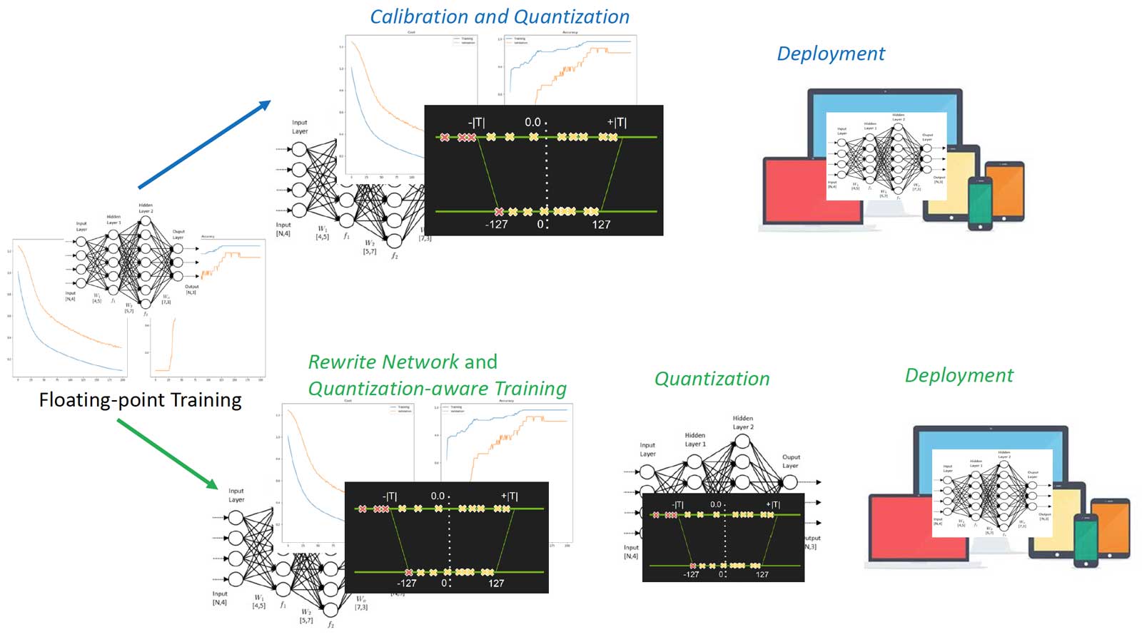
Given a pre-defined full-precision model, the learner inserts quantization nodes and operations into the computation graph of the model. With activation quantization enabled, quantization nodes will also be placed after activation operations (e.g. ReLU).
In the training phase, both full-precision and quantized weights are kept. In the forward pass, quantized weights are obtained by applying the quantization function on full-precision weights. To update full-precision weights in the backward pass, since gradients w.r.t. quantized weights are zeros almost everywhere, we use the straight-through estimator (STE, Bengio et al., 2015) to pass gradients of quantized weights directly to full-precision weights for update.
- Quantized Neural Network PACKage - mobile-optimized implementation of quantized neural network operators
- TensorQuant: A TensorFlow toolbox for Deep Neural Network Quantization
- https://dominikfhg.github.io/TensorQuant/
- https://zhuanlan.zhihu.com/p/38328685
- Distiller is an open-source Python package for neural network compression research.
- Neural Network Quantization
- Neural Network Quantization Resources
- FINN-R: An End-to-End Deep-Learning Framework for Fast Exploration of Quantized Neural Networks
- Making Neural Nets Work With Low Precision
- Differentiable Soft Quantization: Bridging Full-Precision and Low-Bit Neural Networks
- Quantization and Training of Neural Networks for Efficient Integer-Arithmetic-Only Inference
- Lower Numerical Precision Deep Learning Inference and Training
Fixed-point Arithmetic
- A Fixed-Point Arithmetic Package
- http://hackage.haskell.org/package/fixed-point
- https://courses.cs.washington.edu/courses/cse467/08au/labs/l5/fp.pdf
- Fixed Point Arithmetic and Tricks
- Convergence of a Relaxed Variable Splitting Coarse Gradient Descent Method for Learning Sparse Weight Binarized Activation Neural Network
- https://www.math.uci.edu/~jxin/xue.pdf
- https://arxiv.org/abs/1711.07354v1
- https://www.math.uci.edu/~jxin/signals.html
- Extremely Low Bit Neural Network: Squeeze the Last Bit Out with ADMM
- Toward Extremely Low Bit and Lossless Accuracy in DNNs with Progressive ADMM
The state-of-the-art hardware platforms for training Deep Neural Networks (DNNs) are moving from traditional single precision (32-bit) computations towards 16 bits of precision -- in large part due to the high energy efficiency and smaller bit storage associated with using reduced-precision representations. However, unlike inference, training with numbers represented with less than 16 bits has been challenging due to the need to maintain fidelity of the gradient computations during back-propagation. Here we demonstrate, for the first time, the successful training of DNNs using 8-bit floating point numbers while fully maintaining the accuracy on a spectrum of Deep Learning models and datasets. In addition to reducing the data and computation precision to 8 bits, we also successfully reduce the arithmetic precision for additions (used in partial product accumulation and weight updates) from 32 bits to 16 bits through the introduction of a number of key ideas including chunk-based accumulation and floating point stochastic rounding.
- 8-Bit Precision for Training Deep Learning Systems
- Extending 8-bit training breakthroughs to the toughest deep learning models
- Hybrid 8-bit Floating Point (HFP8) Training and Inference for Deep Neural Networks
- Training Deep Neural Networks with 8-bit Floating Point Numbers
- https://www.ibm.com/blogs/research/author/xiao-sun/
Binary neural networks are networks with binary weights and activations at run time. At training time these weights and activations are used for computing gradients; however, the gradients and true weights are stored in full precision. This procedure allows us to effectively train a network on systems with fewer resources.
Forward Binarization
For forward propagation, we need two binary matrices; we thus binarize the weight matrix and the incoming activation from the previous layer.


A key to the success of BNNs it the binary activation function, which clamps all negatives inputs to −1 and all positive inputs to 1. There are two binarized functions:
| deterministic | stochastic |
|---|---|
 |
 |
Here
Gradient Propagation Through Discretization
The derivative of the sign function is zero almost everywhere, making it incompatible with backpropagation. Thus, a straight-through estimator is used. This preserves the gradient's information and cancels large gradients.


While updating the weights, the following is done:
Each real valued weight,
This network has the following layers:

- Fully connected (128)
- Ramp - rectified linear unit (ReLU) activation function
- Binarize activations
- Fully connected (128)
- Ramp - ReLU activation function
- Binarize activations
- Fully connected (10)
- Sigmoid activation function
- https://blog.csdn.net/stdcoutzyx/article/details/50926174
- https://duanyzhi.github.io/Binary-Network/
- BinaryConnect: Training Deep Neural Networks with binary weights during propagations
- Neural Networks with Few Multiplications
- Binary Neural Networks
- Code: Training Deep Neural Networks with Weights and Activations Constrained to +1 or -1
- Code Sample: Optimizing Binarized Neural Networks on Intel® Xeon® Scalable Processors
- Accelerating Neural Networks with Binary Arithmetic
- The High-Dimensional Geometry of Binary Neural Networks
- Binarized Neural Networks: Training Deep Neural Networks with Weights and Activations Constrained to +1 or -1
- Boolean Circuits are Neural Networks
- FP-BNN: Binarized neural network on FPGA
- Embedded Binarized Neural Networks
- Deep Learning for Real-Time Crime Forecasting and Its Ternarization
- https://www.ibm.com/blogs/research/2019/04/2-bit-precision/
Ternary weight networks (TWNs) is the neural networks with weights
constrained to +1, 0 and -1.
This network can date up to the paper Learning algorithms with neural network with ternary weights in 1988.
- Learning algorithms with neural network with ternary weights
- Ternary Weight Networks
- TBN: Convolutional Neural Network with Ternary Inputs and Binary Weights
- Trained Ternary Quantization
- https://iceory.github.io/2018/04/04/ternary-weight-networks/
- https://ieeexplore.ieee.org/document/8581485
In Binary-WeightNetworks, the filters are approximated with binary values resulting in 32× memory saving. In XNOR-Networks, both the filters and the input to convolutional layers are binary. XNOR-Networks approximate convolutions using primarily binary operations. This results in 58× faster convolutional operations and 32× memory savings.

- XNOR-Net: ImageNet Classification Using Binary Convolutional Neural Networks
- GXNOR-Net: Training deep neural networks with ternary weights and activations without full-precision memory under a unified discretization framework
- XNOR-Net: ImageNet Classification Using Binary Convolutional Neural Networks
- Joseph Chet Redmon: author of XORNet
- XNOR-Net论文解读
- https://github.com/liuzechun/Bi-Real-net
- http://iis-projects.ee.ethz.ch/index.php/Bringing_XNOR-nets_(ConvNets)_to_Silicon
- http://web.eng.tau.ac.il/deep_learn/wp-content/uploads/2017/03/Binary-Deep-Learning.pdf
- https://papers.nips.cc/paper/6638-towards-accurate-binary-convolutional-neural-network.pdf
- https://arxiv.org/pdf/2001.05936v1.pdf
- Low Precision Arithmetic Simulation in PyTorch
- Deep Learning with Limited Numerical Precision
- Making Neural Nets Work With Low Precision
- 8-bit Inference with TensorRT
- Decrease the required amount of memory. Half-precision floating point format (FP16) uses 16 bits, compared to 32 bits for single precision (FP32). Lowering the required memory enables training of larger models or training with larger minibatches.
- Shorten the training or inference time. Execution time can be sensitive to memory or arithmetic bandwidth. Half-precision halves the number of bytes accessed, thus reducing the time spent in memory-limited layers.

The Y-axis is the percentage of all values on a log scale. The X-axis is the log scale of absolute values, as well as a special entry for zeros. For example, in this training session 66.8% of values were zero, whereas 4% of values were between
Additions to the traditional iteration procedure are in bold.
- Make an FP16 copy of the weights
- Forward propagate using FP16 weights and activations
- Multiply the resulting loss by the scale factor S
- Backward propagate using FP16 weights, activations, and their gradients
- Multiply the weight gradients by 1/S
- Optionally process the weight gradients (gradient clipping, weight decay, etc.)
- Update the master copy of weights in FP32
- https://nnabla.readthedocs.io/en/latest/python/tutorial/mixed_precision_training.html
- https://nvidia.github.io/OpenSeq2Seq/html/mixed-precision.html
- https://pdc.one/2019/05/14/Mixed-precision-training/
- Paulius Micikevicius's talk "Training Neural Networks with Mixed Precision: Theory and Practice" (GTC 2018, S8923).
- Experimental Evaluation of Mixed Precision Training for End to End Applications
- Apex (A PyTorch Extension)
- https://blog.masterliu.net/tensorflow/tensorflow-mixed-precision/
- Mixed-Precision Training of Deep Neural Networks
- Mixed Precision Training
- User Guide
- TRAINING WITH MIXED PRECISION
- NVIDIA Apex: Tools for Easy Mixed-Precision Training in PyTorch
- https://developer.nvidia.com/vulkan-driver
The convolution in CNN is replaced by the calculating
- https://github.com/huawei-noah/AdderNet
- https://papers.nips.cc/paper/2020/file/1cf44d7975e6c86cffa70cae95b5fbb2-Paper.pdf
- Kernel Based Progressive Distillation for Adder Neural Networks
- https://www.zhihu.com/column/EdgeDeepLearning
- AdderSR: Towards Energy Efficient Image Super-Resolution
- https://arxiv.org/abs/2101.10015
- https://github.com/dlut-dimt/PODM
- A Bridging Framework for Model Optimization and Deep Propagation
Coarse gradient is generally not a gradient of any function but an artificial ascent direction. The weight update of BCGD goes by coarse gradient correction of a weighted average of the full-precision weights and their quantization (the so-called blending), which yields sufficient descent in the objective value and thus accelerates the training.
- https://www.math.uci.edu/~jxin/
- Blended coarse gradient descent for full quantization of deep neural networks
- Training Quantized Deep Neural Networks and Applications with Blended Coarse Gradient Descent
- Blended Coarse Gradient Descent for Full Quantization of Deep Neural Networks
- https://dominikfhg.github.io/TensorQuant/
- Quantized Neural Networks: Training Neural Networks with Low Precision Weights and Activations
- Median Binary-Connect Method and a Binary Convolutional Neural Nework for Word Recognition
- BinaryConnect: Training Deep Neural Networks with binary weights during propagations
- Binary Relax: A Relaxation Approach For Training Deep Neural Networks With Quantized Weights
- Quantization and Training of Low Bit-Width Convolutional Neural Networks for Object Detectio
- https://www.math.uci.edu/~jxin/signals.html
- https://www.researchgate.net/scientific-contributions/43925792_Dimitris_S_Papailiopoulos
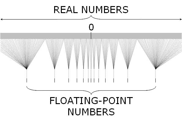
It turns out that DNNs can work with smaller datatypes, with less precision, such as 8-bit integers. Roughly speaking, we’re trying to work with a number line looking closer to the sparse one on the bottom. The numbers are quantized, i.e. discretized to some specific values, which we can then represent using integers instead of floating-point numbers.
- https://arxiv.org/abs/1906.03193
- https://arxiv.org/abs/1903.05662
- https://arxiv.org/pdf/1609.07061.pdf
High-accuracy low precision (HALP) is our algorithm which runs SVRG and uses bit centering with a full gradient at every epoch to update the low-precision representation. It can do better than previous algorithms because it reduces the two sources of noise that limit the accuracy of low-precision SGD: gradient variance and round-off error.
- To reduce noise from gradient variance, HALP uses a known technique called
stochastic variance-reduced gradient (SVRG). SVRG periodically uses full gradients to decrease the variance of the gradient samples used in SGD. - To reduce noise from quantizing numbers into a low-precision representation, HALP uses a new technique we call
bit centering. The intuition behind bit centering is that as we get closer to the optimum, the gradient gets smaller in magnitude and in some sense carries less information, so we should be able to compress it. By dynamically re-centering and re-scaling our low-precision numbers, we can lower the quantization noise as the algorithm converges.
- High-Accuracy Low-Precision Training
- Training deep neural networks with low precision multiplications
- HALP: High-Accuracy Low-Precision Training
There are three primary challenges that make it difficult to scale precision below 16 bits while fully preserving model accuracy. Firstly, when all the operands (i.e., weights, activations, errors, and gradients) for general matrix multiplication (GEMM) and convolution computations are simply reduced to 8 bits, most DNNs suffer noticeable accuracy degradation. Secondly, reducing the bit precision of accumulations in GEMM from 32 bits to 16 bits significantly impacts the convergence of DNN training. This is why commercially available hardware platforms exploiting scaled precision for training (including GPUs) still continue to use 32 bits of precision for accumulation. Reducing accumulation bit precision below 32 bits is critically important for reducing the area and power of 8-bit hardware. Finally, reducing the bit precision of weight updates to 16-bit floating-point impacts accuracy, while 32-bit weight updates, used in today’s systems, require an extra copy of the high-precision weights and gradients to be kept in memory, which is expensive.
- Accumulation Bit-Width Scaling For Ultra-Low Precision Training Of Deep Networks
- Ultra-Low-Precision Training of Deep Neural Networks
- 8-Bit Precision for Training Deep Learning Systems
- Training High-Performance and Large-Scale Deep Neural Networks with Full 8-bit Integers
- Highly Accurate Deep Learning Inference with 2-bit Precision
- OptQuant: Distributed training of neural networks with optimized quantization mechanisms
- https://www.ibm.com/blogs/research/author/chia-yuchen/
- https://www.ibm.com/blogs/research/author/naigangwang/
We can apply alteranting direction method of mulipliers(ADMM) to train deep neural networks. The first part of ADMM-NN is a systematic, joint framework of DNN weight pruning and quantization using ADMM. It can be understood as a smart regularization technique with regularization target dynamically updated in each ADMM iteration, thereby resulting in higher performance in model compression than prior work. The second part is hardware-aware DNN optimizations to facilitate hardware-level implementations. Without accuracy loss, we can achieve 85\timesand 24\timespruning on LeNet-5 and AlexNet models, respectively, significantly higher than prior work. The improvement becomes more significant when focusing on computation reductions. Combining weight pruning and quantization, we achieve 1,910\timesand 231\timesreductions in overall model size on these two benchmarks, when focusing on data storage. Highly promising results are also observed on other representative DNNs such as VGGNet and ResNet-50.
- https://web.northeastern.edu/yanzhiwang/publications/
- Deep ADMM-Net for Compressive Sensing MRI
- Extremely Low Bit Neural Network: Squeeze the Last Bit Out with ADMM
- Toward Extremely Low Bit and Lossless Accuracy in DNNs with Progressive ADMM
- ADMM-based Weight Pruning for Real-Time Deep Learning Acceleration on Mobile Devices
- ADMM-NN: An Algorithm-Hardware Co-Design Framework of DNNs Using Alternating Direction Method of Multipliers
- StructADMM: A Systematic, High-Efficiency Framework of Structured Weight Pruning for DNNs
- https://blog.csdn.net/XSYYMY/article/details/81904882
- https://arxiv.org/abs/1706.06197
- https://csyhhu.github.io/
- https://www.ntu.edu.sg/home/sinnopan/
- https://ywang393.expressions.syr.edu/
- https://cse.buffalo.edu/~wenyaoxu/
- http://gr.xjtu.edu.cn/web/jiansun/publications
Transfer learning methods have demonstrated state-of-the-art performance on various small-scale image classification tasks. This is generally achieved by exploiting the information from an ImageNet convolution neural network (ImageNet CNN). However, the transferred CNN model is generally with high computational complexity and storage requirement. It raises the issue for real-world applications, especially for some portable devices like phones and tablets without high-performance GPUs. Several approximation methods have been proposed to reduce the complexity by reconstructing the linear or non-linear filters (responses) in convolutional layers with a series of small ones.
- EfficientNet: Rethinking Model Scaling for Convolutional Neural Networks
- MobileNets: Efficient Convolutional Neural Networks for Mobile Vision Applications
- Compact Convolutional Neural Network Transfer Learning For Small-Scale Image Classification
- https://zhuanlan.zhihu.com/p/35405071
- https://www.jianshu.com/u/4a95cf020626
- https://github.com/MG2033/ShuffleNet
Note that the deep learning models are composite of linear and non-linear maps. And linear maps are based on matrices.
These methods take a layer and decompose it into several smaller layers. Although there will be more layers after the decomposition, the total number of floating point operations and weights will be smaller. Some reported results are on the order of x8 for entire networks (not aimed at large tasks like imagenet, though), or x4 for specific layers inside imagenet. My experience was that with these decompositions I was able to get a speedup of between x2 to x4, depending on the accuracy drop I was willing to take.
- http://www.tensorlet.com/
- Optimal Low Rank Tensor Factorization for Deep Learning
- https://github.com/jacobgil/pytorch-tensor-decompositions
- Accelerating deep neural networks with tensor decompositions
- Workshop: “Deep Learning and Tensor/Matrix Decomposition for Applications in Neuroscience”, November 17th, Singapore
- http://www.deeptensor.ml/index.html
- http://tensorly.org/stable/home.html
- http://www.vision.jhu.edu/
- https://wabyking.github.io/talks/DL_tensor.pdf
Singular value decomposition
The matrix
To explore a low-rank subspace combined with a sparse structure for the weight matrix
And Toeplitz Matrix can be applied to approximate the weight matrix
$$
W = {\alpha}1T{1}T^{−1}{2} + {\alpha}2 T_3 T{4}^{-1} T{5}
$$
where

- https://en.wikipedia.org/wiki/Low-rank_approximation
- Low Rank Matrix Approximation
- On Compressing Deep Models by Low Rank and Sparse Decomposition
- ESPNets for Computer Vision Efficient CNNs for Edge Devices
- https://www.cnblogs.com/zhonghuasong/p/7821170.html
- https://github.com/chester256/Model-Compression-Papers
- https://arxiv.org/pdf/1712.01887.pdf
- https://srdas.github.io/DLBook/intro.html#effective
- https://cognitiveclass.ai/courses/accelerating-deep-learning-gpu/
- https://github.com/songhan/Deep-Compression-AlexNet
- awesome-model-compression-and-acceleration
- gab41.lab41.org
- CS 598 LAZ: Cutting-Edge Trends in Deep Learning and Recognition
- http://slazebni.cs.illinois.edu/spring17/lec06_compression.pdf
- http://slazebni.cs.illinois.edu/spring17/reading_lists.html#lec06
- CS236605: Deep Learning
- https://mlperf.org/
All techniques above can be used to fully-connected networks or generally feed-forward network. RNN is feedback network where there is rings in its computational graph.

- Dynamically Hierarchy Revolution: DirNet for Compressing Recurrent Neural Network on Mobile Devices
- Compressing Recurrent Neural Network with Tensor Train
- Learning Compact Recurrent Neural Networks with Block-Term Tensor Decomposition
- ANTMAN: SPARSE LOW-RANK COMPRESSION TO ACCELERATE RNN INFERENCE
- Deep Compresion
- Run-Time Efficient RNN Compression for Inference on Edge Devices
- LSTM compression for language modeling
- Parameter Compression of Recurrent Neural Networks and Degradation of Short-term Memory
- https://ai.google/research/pubs/pub44632
- CLINK: Compact LSTM Inference Kernel for Energy Efficient Neurofeedback Devices
- https://arxiv.org/abs/1902.00159
- https://github.com/mit-han-lab/gan-compression
- https://hanlab.mit.edu/projects/gancompression/
- https://github.com/amitadate/gan-compression
- Adversarial Network Compression
- Model Compression with Generative Adversarial Networks
- https://github.com/kedartatwawadi/NN_compression
- Optimizing Data-Intensive Computations in Existing Libraries with Split Annotations
- https://github.com/khakhulin/compressed-transformer
- http://nla.skoltech.ru/projects/files/presentations/team_21.pdf
- https://shaojiejiang.github.io/post/en/compressive-transformers/
- https://github.com/khakhulin/compressed-transformer
- https://github.com/szhangtju/The-compression-of-Transformer
- https://github.com/intersun/PKD-for-BERT-Model-Compression
- https://huggingface.co/transformers/model_doc/mobilebert.html

- https://www.cse.wustl.edu/~ychen/HashedNets/
- Compressing Neural Networks with the Hashing Trick
- https://spectrum.ieee.org/tech-talk/computing/hardware/algorithms-and-hardware-for-deep-learning
- https://www2021.thewebconf.org/papers/hashing-accelerated-graph-neural-networks-for-link-prediction/
The problem of deep learning
Sometimes we need partition the model or the data into different machines. In another world, the model or the data are distributed in a few machines.
Distributed training of deep learning models is a branch of distributed computation.
Training advanced deep learning models is challenging. Beyond model design, model scientists also need to set up the state-of-the-art training techniques such as distributed training, mixed precision, gradient accumulation, and checkpointing. Yet still, scientists may not achieve the desired system performance and convergence rate. Large model sizes are even more challenging: a large model easily runs out of memory with pure data parallelism and it is difficult to use model parallelism.
It is really important to reduce the cost of communication in distributed computation including the communication time, communication frequency, communication content and latency.
- https://www.cs.rice.edu/~as143/COMP640_Fall16/
- https://www.cs.rice.edu/~as143/
- https://www.deepspeed.ai/
- https://shivaram.org/
- https://www.comp.hkbu.edu.hk/~chxw/
- High Performance Distributed Deep Learning
- Tutorial: High Performance Distributed Deep Learning
- https://itpeernetwork.intel.com/accelerating-deep-learning-workloads/#gs.ny4nke
- A Generic Communication Scheduler for Distributed DNN Training Acceleration
- https://arxiv.org/pdf/1806.03377.pdf
- http://www.iiswc.org/iiswc2019/index.html
- https://cs.stanford.edu/~matei/
- Bandwidth Optimal All-reduce Algorithms for Clusters of Workstations
- https://zhuanlan.zhihu.com/p/87515411
- https://zhuanlan.zhihu.com/p/84862107
- Accelerating Deep Learning Workloads through Efficient Multi-Model Execution
- Multi-tenant GPU Clusters for Deep Learning Workloads: Analysis and Implications
- https://cs.stanford.edu/~matei/
- Characterizing Deep Learning Training Workloads on Alibaba-PAI
- https://www.microsoft.com/en-us/research/project/fiddle/
- https://github.com/bytedance/byteps
- https://github.com/msr-fiddle/pipedream
- https://github.com/msr-fiddle/philly-trace
- https://www.microsoft.com/en-us/research/project/fiddle/
- PipeMare: Asynchronous Pipeline Parallel DNN Training
- GPipe: Efficient Training of Giant Neural Networks using Pipeline Parallelism
- XPipe: Efficient Pipeline Model Parallelism for Multi-GPU DNN Training
- https://arxiv.org/pdf/1806.03377.pdf
- Multi-tenant GPU Clusters for Deep Learning Workloads: Analysis and Implications
- PipeDream: Generalized Pipeline Parallelism for DNN Training
AdaptDL is a resource-adaptive deep learning (DL) training and scheduling framework. The goal of AdaptDL is to make distributed DL easy and efficient in dynamic-resource environments such as shared clusters and the cloud.
The communication cost of distributed training depends on the content which the distributed machines share.
- https://www.usenix.org/conference/hotedge18/presentation/tao
- eSGD: Communication Efficient Distributed Deep Learning on the Edge
- https://www.run.ai/
- https://theaisummer.com/distributed-training/
- Communication-Efficient Learning of Deep Networks from Decentralized Data
- https://www.usenix.org/system/files/conference/atc17/atc17-zhang.pdf
- https://embedl.ai/
- Communication-Efficient Federated Deep Learning With Layerwise Asynchronous Model Update and Temporally Weighted Aggregation
- Optimus: An Efficient Dynamic Resource Scheduler for Deep Learning Clusters
- CS-345, Spring 2019: Advanced Distributed and Networked Systems
- http://www.cs.cmu.edu/~muli/file/parameter_server_nips14.pdf
- http://www1.se.cuhk.edu.hk/~htwai/oneworld/pdf/ji_SP.pdf
- GPU Direct RDMA
The DeepSpeed API is a lightweight wrapper on PyTorch.
This means that you can use everything you love in PyTorch and without learning a new platform.
In addition, DeepSpeed manages all of the boilerplate state-of-the-art training techniques, such as distributed training, mixed precision, gradient accumulation, and checkpoints so that you can focus on your model development.
Most importantly, you can leverage the distinctive efficiency and effectiveness benefit of DeepSpeed to boost speed and scale with just a few lines of code changes to your PyTorch models.
NCCL (pronounced "Nickel") is a stand-alone library of standard communication routines for GPUs, implementing all-reduce, all-gather, reduce, broadcast, reduce-scatter, as well as any send/receive based communication pattern. It has been optimized to achieve high bandwidth on platforms using PCIe, NVLink, NVswitch, as well as networking using InfiniBand Verbs or TCP/IP sockets. NCCL supports an arbitrary number of GPUs installed in a single node or across multiple nodes, and can be used in either single- or multi-process (e.g., MPI) applications.
- https://github.com/NVIDIA/nccl
- https://docs.nvidia.com/deeplearning/sdk/nccl-developer-guide/index.html
Gradient code and compression is to accelerate the distributed training of deep learning models by reducing the communication cost.
Some nodes may be much slower than others parallelized or distributed computation enviroment. With redundancy, we may not need every node to finish. See prior articles for more areticles on this topic.
Approximate gradient coding allows us to tolerate more stragglers with less work.
- Gradient Coding
- Reducing the Average Delay in Gradient Coding
- Tree Gradient Coding
- Communication-computation efficient gradient coding
- Approximate Gradient Coding via Sparse Random Graphs
- ErasureHead: Distributed Gradient Descent without Delays Using Approximate Gradient Coding
- https://users.oden.utexas.edu/~leiqi/stragglers_nips.pdf
- https://zachcharles.com/files/Presentations/sbc_slides.pdf
- Ternary Gradients to Reduce Communication in Distributed Deep Learning (TensorFlow)
- https://hwang595.github.io/publications/
- http://papail.io/
- http://kangwooklee.com/
- https://www.ntu.edu.sg/home/hmkiah/
- https://users.oden.utexas.edu/~leiqi/
- https://zachcharles.com/
In distributed training of machine learning models with stochastic optimization, the exchange of parameter updates between workers often is a bottleneck that limits the scalability of distributed training.
This is especially true for models with a large parameter space, such as neural networks.
Several techniques have been proposed to enhance scalability by compressing gradients,
e.g. by sending a sparse set of coordinates only, or by quantization.
We study the gradient compression literature from both sides: on the one hand, we study properties of these algorithms in a distributed setting, and their effectiveness for speed and scalability. On the other hand, we explore properties of the minima found by these algorithms, such as robustness or generalisation.
- Deep Gradient Compression: Reducing the Communication Bandwidth for Distributed Training
- https://blog.csdn.net/a609640147/article/details/90054754
- https://songhan.mit.edu/
- Deep Leakage from Gradients
- https://littleorange.site/2019/02/deep-gradient-compression.html
- Training Kinetics in 15 Minutes: Large-scale Distributed Training on Videos
We study gradient compression methods to alleviate the communication bottleneck in data-parallel distributed optimization. Despite the significant attention received, current compression schemes either do not scale well or fail to achieve the target test accuracy. We propose a new low-rank gradient compressor based on power iteration that can i) compress gradients rapidly, ii) efficiently aggregate the compressed gradients using all-reduce, and iii) achieve test performance on par with SGD. The proposed algorithm is the only method evaluated that achieves consistent wall-clock speedups when benchmarked against regular SGD with an optimized communication backend. We demonstrate reduced training times for convolutional networks as well as LSTMs on common datasets.
- Gradient Compression Techniques to Accelerate Distributed Training of Neural Networks
- QSGD: Communication-Efficient SGD via Gradient Quantization and Encoding
- Sparse Binary Compression: Towards Distributed Deep Learning with minimal Communication
- ATOMO: Communication-efficient Learning via Atomic Sparsification
- Error Feedback Fixes SignSGD and other Gradient Compression Schemes
- https://github.com/epfml/error-feedback-SGD
- PowerSGD: Practical Low-Rank Gradient Compression for Distributed Optimization
- https://github.com/epfml/powersgd
- Decentralized SGD and Consensus with Communication Compression
- https://sstich.ch/
- https://tvogels.nl/
- https://parsa.epfl.ch/~falsafi/
- https://lts4.epfl.ch/people/people-current/frossard-2/
- http://www.martinjaggi.ch/
- http://www.sysml.cc/
- https://sstich.ch/
- https://www.epfl.ch/labs/mlo/
- Sparse Communication for Distributed Gradient Descent
- https://www.kheafield.com/
- https://www.kheafield.com/papers/
- http://fusharblog.com/archive/
- Gradient compression for distributed training of machine learning models
- https://www.maths.ed.ac.uk/~prichtar/i_papers.html
- https://richtarik.org/i_papers.html
- https://richtarik.org/i_team.html
- https://www.maths.ed.ac.uk/~prichtar/i_seminar.html
- Better Communication Complexity for Local SGD
- Gradient Descent with Compressed Iterates
Sketch is a class of algorithms using a probabilistic data structure to approximate the distribution of input data.
The count-sketches streaming algorithm instantiates the following framework:
- Find a randomized streaming algorithm whose output (as a random variable) has the desired expectation but usually high variance (i.e., noise).
- To reduce the variance/noise, run many independent copies in parallel and combine their outputs.
- Compressing Gradient Optimizers via Count-Sketches
- MISSION: Ultra Large-Scale Feature Selection using Count-Sketches
- Buffered Count-Min Sketch on SSD: Theory and Experiments
- https://github.com/rdspring1/Count-Sketch-Optimizers
- http://net.pku.edu.cn/~yangtong/
- https://dblp.org/pers/hd/k/Kyrillidis:Anastasios
- https://www.csauthors.net/vijai-mohan/
- SketchML: Accelerating Distributed Machine Learning with Data Sketches
It’s a simple idea: rather than compute gradients through backpropagation, we can train a model to predict what those gradients will be, and use our prediction to update our weights. It’s dynamic programming for neural networks.
- https://github.com/andrewliao11/dni.pytorch
- Understanding Synthetic Gradients and Decoupled Neural Interfaces
- Synthetic Gradients with Tensorflow
- http://deliprao.com/archives/187
- Exploring the Use of Synthetic Gradients for Distributed Deep Learning across Cloud and Edge Resources
- Decoupled Neural Interfaces using Synthetic Gradients
- http://cnichkawde.github.io/SyntheticGradients.html
- A Bird's Eye View of Synthetic Gradients
- https://iamtrask.github.io/2017/03/21/synthetic-gradients/
Gradient Centralization (GC) is a simple and effective optimization technique for Deep Neural Networks (DNNs), which operates directly on gradients by centralizing the gradient vectors to have zero mean. It can both speedup training process and improve the final generalization performance of DNNs.
- http://www.breloff.com/
- https://github.com/Yonghongwei/Gradient-Centralization- Gradient Centralization: A New Optimization Technique for Deep Neural Networks
Ranger now uses Gradient Centralization by default, and applies it to all conv and fc layers by default. However, everything is customizable so you can test with and without on your own datasets. (Turn on off via "use_gc" flag at init).
- Ranger - a synergistic optimizer combining RAdam (Rectified Adam) and LookAhead, and now GC (gradient centralization) in one optimization
- https://github.com/lessw2020/Ranger-Mish-ImageWoof-5
Existing security mechanisms for high-performance and distributed computing infrastructure are complex and difficult to deploy.
As a result, many high-performance and distributed computing facilities do no deploy sufficient security mechanisms.
This has prevented privacy-sensitive applications, such as those in the medical fields, and security-sensitive applications from using such facilities.
In this project, we will develop and deploy DICE, Data Insurance in the Cluster Environment, to enhance the security in HPC and distributed computing clusters.
DICE will consist of three major components: a container-based virtual cluster, a component to defend against side-channel attacks, and a secure execution ledger for auditing.
The container-based virtual cluster will be developed based on the Docker Linux container.
The Docker security mechanism will be enhanced by deploying an effective key management scheme for groups and by reducing the attack surface exposed to containers.
Novel defense mechanisms will be developed and deployed to defend against side-channel attacks in the cluster environment by exploiting new security features in the recent processors.
The secure execution ledger will provide a global holistic view of program execution in the whole system, enabling auditing the behavior of individual user as well as user groups.
DICE essentially creates a two-level security model: on the (physical) cluster level, a group of (mostly) mutually trusted users share a single virtual cluster for their jobs; and inside the virtual cluster, the group may use existing security mechanisms of their software-of-choice to further refine security.
- https://github.com/amplab/drizzle-spark
- https://github.com/horovod/horovod
- http://maxpumperla.com/elephas/
- https://horovod.ai/
- http://explorer.cs.fsu.edu/
BigDL is a distributed deep learning library for Apache Spark; with BigDL, users can write their deep learning applications as standard Spark programs, which can directly run on top of existing Spark or Hadoop clusters. To makes it easy to build Spark and BigDL applications, a high level Analytics Zoo is provided for end-to-end analytics + AI pipelines.
- BigDL is a distributed deep learning library for Apache Spark
- https://github.com/intel-analytics/BigDL/
Drizzle is a low latency execution engine for Apache Spark that is targeted at stream processing and iterative workloads. Currently, Spark uses a BSP computation model, and notifies the scheduler at the end of each task. Invoking the scheduler at the end of each task adds overheads and results in decreased throughput and increased latency.
Horovod can additionally run on top of Apache Spark, making it possible to unify data processing and model training into a single pipeline. Once Horovod has been configured, the same infrastructure can be used to train models with any framework, making it easy to switch between TensorFlow, PyTorch, MXNet, and future frameworks as machine learning tech stacks continue to evolve.
Elephas is an extension of Keras, which allows you to run distributed deep learning models at scale with Spark.
- https://zhuanlan.zhihu.com/p/87392811
- https://zhuanlan.zhihu.com/p/87458316
- https://www.dataiku.com/
- https://www.fritz.ai/
- TensorFlow: Large-Scale Machine Learning on Heterogeneous Distributed Systems
- PyTorch: An Imperative Style, High-Performance Deep Learning Library
TensorFlow is an end-to-end open source platform for machine learning. It has a comprehensive, flexible ecosystem of tools, libraries, and community resources that lets researchers push the state-of-the-art in ML and developers easily build and deploy ML-powered applications.
- https://www.tensorflow.org/resources/tools
- https://github.com/tensorflow/tensorflow
- https://www.tensorflow.org/lite?hl=zh-cn
- https://github.com/tensorflow/tflite-support
PyTorch is a Python package that provides two high-level features:
- Tensor computation (like NumPy) with strong GPU acceleration
- Deep neural networks built on a tape-based autograd system
PyTorch has minimal framework overhead. We integrate acceleration libraries such as Intel MKL and NVIDIA (cuDNN, NCCL) to maximize speed. At the core, its CPU and GPU Tensor and neural network backends (TH, THC, THNN, THCUNN) are mature and have been tested for years.
Hence, PyTorch is quite fast – whether you run small or large neural networks.
The memory usage in PyTorch is extremely efficient compared to Torch or some of the alternatives. We've written custom memory allocators for the GPU to make sure that your deep learning models are maximally memory efficient. This enables you to train bigger deep learning models than before.
- https://pytorch.org/
- https://github.com/pytorch/pytorch
- https://pytorch-lightning.readthedocs.io/en/0.5.3.2/Trainer/Distributed%20training/
- https://pytorch.org/mobile/home/
- https://github.com/rusty1s/pytorch_geometric
PaddlePaddle, as the only independent R&D deep learning platform in China, has been officially open-sourced to professional communities since 2016. It is an industrial platform with advanced technologies and rich features that cover core deep learning frameworks, basic model libraries, end-to-end development kits, tools & components as well as service platforms. PaddlePaddle is originated from industrial practices with dedication and commitments to industrialization. It has been widely adopted by a wide range of sectors including manufacturing, agriculture, enterprise service, and so on while serving more than 2.3 million developers. With such advantages, PaddlePaddle has helped an increasing number of partners commercialize AI.
MindSpore is a new open source deep learning training/inference framework that could be used for mobile, edge and cloud scenarios. MindSpore is designed to provide development experience with friendly design and efficient execution for the data scientists and algorithmic engineers, native support for Ascend AI processor, and software hardware co-optimization. At the meantime MindSpore as a global AI open source community, aims to further advance the development and enrichment of the AI software/hardware application ecosystem.
- https://github.com/mindspore-ai/mindspore
- https://www.mindspore.cn/
- https://gitee.com/mindspore/mindspore
MegEngine is a fast, scalable and easy-to-use deep learning framework, with auto-differentiation.
- https://megengine.org.cn/
- https://www.openi.org.cn/html/2020/Framework_0325/18.html
- https://github.com/MegEngine/MegEngine
Oneflow is an open source deep learning platform with whole new frame design and the world's leading technology for distributed system.
Darknet is an open source neural network framework written in C and CUDA. It is fast, easy to install, and supports CPU and GPU computation.
Edge computation is to perform some computation on the edge devices such as the monior in order to send less raw data to the computation center.
Machine learning models for edge devices need to have a small footprint in terms of storage, prediction latency, and energy. One instance of where such models are desirable is resource-scarce devices and sensors in the Internet of Things (IoT) setting. Making real-time predictions locally on IoT devices without connecting to the cloud requires models that fit in a few kilobytes.
- https://github.com/microsoft/EdgeML
- https://github.com/fritzlabs/Awesome-Mobile-Machine-Learning
- https://github.com/Bisonai/awesome-edge-machine-learning
- https://github.com/hoangcuong2011/Good-Papers
- https://github.com/rkirkendall/MLEdgeDeploy
- https://github.com/sig-ml/bleedml
- https://www.usenix.org/conference/hotedge18
- https://project-sparthan.github.io/
Mobile deep learning is aimed to run deep learning models (training or inference) on the mobile phones.
It is necessary to compress the deep learning models in order to run it in mobile phones.
- https://www.fritz.ai/resources/mobile-ml-github-repositories.html
- https://www.sigmobile.org/mobisys/2019/workshops/deepmobile19/
- https://github.com/amusi/mobile-deep-learning
- https://github.com/pytorch/qnnpack
- https://mi.inf.ed.ac.uk/
- https://www-users.cs.umn.edu/~fengqian/
- http://homepages.inf.ed.ac.uk/ppatras/
- https://www.cs.ucr.edu/~jiasi/
- https://ix.cs.uoregon.edu/~jiao/
- https://arxiv.org/abs/1904.09274
- https://www.zhqiang.org/deep-learning-mobile/
- https://bdtechtalks.com/2019/12/30/computer-vision-applications-deep-learning/
- MuffNet: Multi-Layer Feature Federation for Mobile Deep Learning
- Deep Learning for Mobile Multimedia: A Survey
- https://github.com/pytorch/qnnpack
- https://github.com/PaddlePaddle/Paddle-Lite
- https://paddlepaddle.github.io/Paddle-Lite/
- https://github.com/alibaba/MNN
- https://www.tensorflow.org/lite
- https://project-sparthan.github.io/papers/acm19.pdf
- https://github.com/XiaoMi/mace
- https://mace.readthedocs.io/en/latest/
- https://github.com/OAID/Tengine
- https://github.com/OAID/Tengine
- https://github.com/onnx/onnx
- https://developer.nvidia.com/tensorrt-getting-started
- https://catalog.ngc.nvidia.com/orgs/nvidia/containers/pytorch
- https://github.com/facebookincubator/AITemplate
MNN is a highly efficient and lightweight deep learning framework. It supports inference and training of deep learning models, and has industry leading performance for inference and training on-device. At present, MNN has been integrated in more than 20 apps of Alibaba Inc, such as Taobao, Tmall, Youku, Dingtalk, Xianyu and etc., covering more than 70 usage scenarios such as live broadcast, short video capture, search recommendation, product searching by image, interactive marketing, equity distribution, security risk control. In addition, MNN is also used on embedded devices, such as IoT.
TNN is a high-performance and lightweight inference framework for mobile devices. It provides lots of advanced features such as cross-platform, model-compression, and code-pruning. TNN, inspired by mainstream open-source industry frameworks, integrates and leverages Youtu Lab's Rapidnet, ncnn framework.
ncnn is a high-performance neural network inference computing framework optimized for mobile platforms. ncnn is deeply considerate about deployment and uses on mobile phones from the beginning of design. ncnn does not have third party dependencies. it is cross-platform, and runs faster than all known open source frameworks on mobile phone cpu. Developers can easily deploy deep learning algorithm models to the mobile platform by using efficient ncnn implementation, create intelligent APPs, and bring the artificial intelligence to your fingertips. ncnn is currently being used in many Tencent applications, such as QQ, Qzone, WeChat, Pitu and so on.
- https://www.wandb.com/
- https://github.com/fastnlp/fitlog
- https://optuna.org/
- https://preferred.jp/en/projects/optuna/
- https://lutzroeder.github.io/netron/
- https://netron.app/
- https://github.com/lutzroeder/netron
- https://github.com/onnx/onnx
- https://github.com/daquexian/onnx-simplifier
- https://github.com/drcut/CPD
- https://github.com/purine/purine2
- https://dlonsc19.github.io/
- http://prace.it4i.cz/en/HPDDL-01-2018