[TOC]
IoU(Intersection over Union),又称重叠度/交并比。
1 NMS:当在图像中预测多个proposals、pred bboxes时,由于预测的结果间可能存在高冗余(即同一个目标可能被预测多个矩形框),因此可以过滤掉一些彼此间高重合度的结果;具体操作就是根据各个bbox的score降序排序,剔除与高score bbox有较高重合度的低score bbox,那么重合度的度量指标就是IoU;
2 mAP:得到检测算法的预测结果后,需要对pred bbox与gt bbox一起评估检测算法的性能,涉及到的评估指标为mAP,那么当一个pred bbox与gt bbox的重合度较高(如IoU score > 0.5),且分类结果也正确时,就可以认为是该pred bbox预测正确,这里也同样涉及到IoU的概念;
提到IoU,大家都知道怎么回事,讲起来也都头头是道,我拿两个图示意下(以下两张图都不是本人绘制):
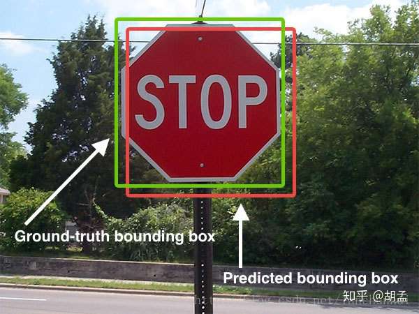
绿框:gt bbox;
红框:pred bbox;
那么IoU的计算如下:
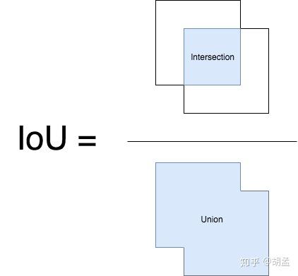
简单点说,就是gt bbox、pred bbox交集的面积 / 二者并集的面积;
好了,现在理解IoU的原理和计算方法了,就应该思考如何函数实现了,这也是我写本笔记的原因;
有次面试实习生的时候,一位同学讲各类目标检测算法头头是道,说到自己复现某某算法的mAP高达多少多少,问完他做的各种改进后,觉得小伙子还是挺不错的;
后来我是想着问问mAP的概念吧,但又觉得有点太复杂,不容易一下讲清楚细节,那就问问IoU吧,结果那位小朋友像傻逼一样看着我,说就是两个bbox的交并比啊,我说那要不你写段伪代码实现下吧,既然简单的话,应该实现起来还是很快的(一般我们也都会有这么个写伪代码的面试步骤,考考动手能力和思考能力吧);然后那位自信满满的小伙子就立马下手开始写了,一般听完题目直接写代码的面试者,有两种可能性:
1 确实写过类似的代码,已经知道里面有哪些坑了,直接信手拈来;
2 没写过类似的代码,且把问题考虑简单化了;
我说你不用着急写,可以先想想两个bbox出现交集的各种情况,如两个bbox如何摆放,位置,以及二者不存在交集的情况等等(看到IoU的具体代码后,你会发现虽然只有寥寥几行代码,但其实已经处理好此类情况了),然后他画了几个图,瞬间表情严肃起来,然后我继续说你还得考虑一个bbox包围另一个bbox;两bbox并不是边角相交,而是两条边相交的特殊情况等等(说到这里我觉得自己也坏坏滴,故意把人家往歪路上牵。。。但主要是看得出来他确实不熟悉IoU的实现了),他就又画了若干种情况,最后开始写代码,刚开始还ok,写了十几行,后来越加越多,草稿纸上也涂涂改改越来越夸张,脸也越胀越红;我看了下他的代码,觉得他思路还行,考虑的还挺周全的,就给了他一个提示:你有没有考虑到你列举的这些情况,有一些可以合并的?他看了下,觉得是可以合并一些情况,就删减了部分代码,稿纸上就更乱了,然后又问他:可不可以继续合并;他就又继续思考了。。。大概是后来越想越复杂,就给我说这个原理他懂的,代码也看过,但现在确实是没能写出来;然后我安慰他,说如果没写过的话,确实是会把问题考虑简单化 / 复杂化,不过我并不是专门考个题目刁难你,而是因为你一直都在做目标检测,所以以为IoU的原理、实现你应该会比较熟悉的,写起代码也应该没问题的;而且你的思路也挺好的,先考虑各种复杂情况,再慢慢合并一些情况,先从1到N,再回到1就行,只不过可能到了N,没考虑到如何再回到1了;
再后来,也面试过其他实习生同学,问到了IoU的实现,很可惜,好像还没有一位同学能圆满写出来的。。。当然了,可能是我有时候过于抠细节了,不利于他们的发挥吧。。。
好了,以上都是废话,看看如何实现吧;
# -*- coding: utf-8 -*-
#
# This is the python code for calculating bbox IoU,
# By running the script, we can get the IoU score between pred / gt bboxes
#
# Author: hzhumeng01 2018-10-19
# copyright @ netease, AI group

from __future__ import print_function, absolute_import
import numpy as np

def get_IoU(pred_bbox, gt_bbox):
    """
    return iou score between pred / gt bboxes
    :param pred_bbox: predict bbox coordinate
    :param gt_bbox: ground truth bbox coordinate
    :return: iou score
    """

    # bbox should be valid, actually we should add more judgements, just ignore here...
    # assert ((abs(pred_bbox[2] - pred_bbox[0]) > 0) and
    #         (abs(pred_bbox[3] - pred_bbox[1]) > 0))
    # assert ((abs(gt_bbox[2] - gt_bbox[0]) > 0) and
    #         (abs(gt_bbox[3] - gt_bbox[1]) > 0))

    # -----0---- get coordinates of inters
    ixmin = max(pred_bbox[0], gt_bbox[0])
    iymin = max(pred_bbox[1], gt_bbox[1])
    ixmax = min(pred_bbox[2], gt_bbox[2])
    iymax = min(pred_bbox[3], gt_bbox[3])
    iw = np.maximum(ixmax - ixmin + 1., 0.)
    ih = np.maximum(iymax - iymin + 1., 0.)

    # -----1----- intersection
    inters = iw * ih

    # -----2----- union, uni = S1 + S2 - inters
    uni = ((pred_bbox[2] - pred_bbox[0] + 1.) * (pred_bbox[3] - pred_bbox[1] + 1.) +
           (gt_bbox[2] - gt_bbox[0] + 1.) * (gt_bbox[3] - gt_bbox[1] + 1.) -
           inters)

    # -----3----- iou
    overlaps = inters / uni

    return overlaps


def get_max_IoU(pred_bboxes, gt_bbox):
    """
    given 1 gt bbox, >1 pred bboxes, return max iou score for the given gt bbox and pred_bboxes
    :param pred_bbox: predict bboxes coordinates, we need to find the max iou score with gt bbox for these pred bboxes
    :param gt_bbox: ground truth bbox coordinate
    :return: max iou score
    """

    # bbox should be valid, actually we should add more judgements, just ignore here...
    # assert ((abs(gt_bbox[2] - gt_bbox[0]) > 0) and
    #         (abs(gt_bbox[3] - gt_bbox[1]) > 0))

    if pred_bboxes.shape[0] > 0:
        # -----0---- get coordinates of inters, but with multiple predict bboxes
        ixmin = np.maximum(pred_bboxes[:, 0], gt_bbox[0])
        iymin = np.maximum(pred_bboxes[:, 1], gt_bbox[1])
        ixmax = np.minimum(pred_bboxes[:, 2], gt_bbox[2])
        iymax = np.minimum(pred_bboxes[:, 3], gt_bbox[3])
        iw = np.maximum(ixmax - ixmin + 1., 0.)
        ih = np.maximum(iymax - iymin + 1., 0.)

        # -----1----- intersection
        inters = iw * ih

        # -----2----- union, uni = S1 + S2 - inters
        uni = ((gt_bbox[2] - gt_bbox[0] + 1.) * (gt_bbox[3] - gt_bbox[1] + 1.) +
               (pred_bboxes[:, 2] - pred_bboxes[:, 0] + 1.) * (pred_bboxes[:, 3] - pred_bboxes[:, 1] + 1.) -
               inters)

        # -----3----- iou, get max score and max iou index
        overlaps = inters / uni
        ovmax = np.max(overlaps)
        jmax = np.argmax(overlaps)

    return overlaps, ovmax, jmax

if __name__ == "__main__":

    # test1
    pred_bbox = np.array([50, 50, 90, 100])   # top-left: <50, 50>, bottom-down: <90, 100>, <x-axis, y-axis>
    gt_bbox = np.array([70, 80, 120, 150])
    print (get_IoU(pred_bbox, gt_bbox))

    # test2
    pred_bboxes = np.array([[15, 18, 47, 60],
                          [50, 50, 90, 100],
                          [70, 80, 120, 145],
                          [130, 160, 250, 280],
                          [25.6, 66.1, 113.3, 147.8]])
    gt_bbox = np.array([70, 80, 120, 150])
    print (get_max_IoU(pred_bboxes, gt_bbox))
其实计算bbox间IoU唯一的难点就在计算intersection,代码的实现很简单:
ixmin = max(pred_bbox[0], gt_bbox[0])
iymin = max(pred_bbox[1], gt_bbox[1])
ixmax = min(pred_bbox[2], gt_bbox[2])
iymax = min(pred_bbox[3], gt_bbox[3])
iw = np.maximum(ixmax - ixmin + 1., 0.)
ih = np.maximum(iymax - iymin + 1., 0.)
比较厉害的就是,以上短短六行代码就可以囊括所有pred bbox与gt bbox间的关系,不管是bboxes间相交 / 不相交,各种相交形式等等;我们在画图分析两个bbox间的关系时,会考虑各种情况,动手实践时会发现很复杂,是因为我们陷入了一种先入为主的思维,就是pred bbox与gt bbox有一个先后顺序,即我们认定了pred bbox为画图中的第一个bbox,gt bbox为第二个,这样在二者有不同位置关系时,就得考虑各种坐标判断情况,但若此时交换二者位置,其实并不影响我们计算IoU;
以上六行代码也印证了这个观点,直接计算两个bbox的相交边框坐标即可,若不相交得到的结果中,必有ixmax < ixmin、iymax - iymin其一成立,此时iw、ih就为0了;
好了,以上就是IoU的计算,原理比较简单,具体分析比较复杂,实现却异常简单,但通过对问题的深入分析,也能加深我们对知识的理解;
代码我传到github上了,比较简单:IoU_demo.py
参考资料
Mean Intersection over Union(MIoU,均交并比),为语义分割的标准度量。其计算两个集合的交集和并集之比,在语义分割问题中,这两个集合为真实值(ground truth)和预测值(predicted segmentation)。这个比例可以变形为TP(交集)比上TP、FP、FN之和(并集)。在每个类上计算IoU,然后取平均。 $$ MIoU=\frac{1}{k+1}\sum^{k}{i=0}{\frac{p{ii}}{\sum_{j=0}^{k}{p_{ij}+\sum_{j=0}^{k}{p_{ji}-p_{ii}}}}} $$ pij表示真实值为i,被预测为j的数量。
直观理解

红色圆代表真实值,黄色圆代表预测值。橙色部分为两圆交集部分。
- MPA(Mean Pixel Accuracy,均像素精度):计算橙色与红色圆的比例;
- MIoU:计算两圆交集(橙色部分)与两圆并集(红色+橙色+黄色)之间的比例,理想情况下两圆重合,比例为1。
Tensorflow源码解析
Tensorflow主要用tf.metrics.mean_iou来计算mIoU,下面解析源码:
第一步:计算混淆矩阵
混淆矩阵例子

# 主要代码
def confusion_matrix(labels, predictions, num_classes=None, dtype=dtypes.int32,
                     name=None, weights=None):
    # 例子:labels =     [0, 1, 2, 0, 3]
    #      predictions =[0, 1, 1, 3, 3]
    if num_classes is None: # 不指定类别个数,就以labels或者predictions最大的指定,即4
      num_classes = math_ops.maximum(math_ops.reduce_max(predictions),
                                     math_ops.reduce_max(labels)) + 1
    else:
      num_classes_int64 = math_ops.cast(num_classes, dtypes.int64)
      labels = control_flow_ops.with_dependencies(
          [check_ops.assert_less(
              labels, num_classes_int64, message='`labels` out of bound')],
          labels)
      predictions = control_flow_ops.with_dependencies(
          [check_ops.assert_less(
              predictions, num_classes_int64,
              message='`predictions` out of bound')],
          predictions)

    if weights is not None:
      predictions.get_shape().assert_is_compatible_with(weights.get_shape())
      weights = math_ops.cast(weights, dtype)

    shape = array_ops.stack([num_classes, num_classes])
    indices = array_ops.stack([labels, predictions], axis=1)
    # indices = [[0,0],[1,1],[2,1],[0,3],[3,3]]
    values = (array_ops.ones_like(predictions, dtype)
              if weights is None else weights)
    # 对应位置的values,若不指定,则全为1
    cm_sparse = sparse_tensor.SparseTensor(
        indices=indices, values=values, dense_shape=math_ops.to_int64(shape))
    # 稀疏张量,指定indices位置为指定value,其他位置为0
    # 多次指定一个位置,value为多次相加的结果
    zero_matrix = array_ops.zeros(math_ops.to_int32(shape), dtype)

    return sparse_ops.sparse_add(zero_matrix, cm_sparse)
SparseTensor例子:
import tensorflow as tf
a = tf.SparseTensor(indices=[[0,0], [1,2], [0, 0]], values=[1, 1, 1], dense_shape=[3, 4])
zero_m = array_ops.zeros(math_ops.to_int32([3,4]),dtype=tf.int32)
r = sparse_ops.sparse_add(zero_m, a)
sess = tf.Session(config=tf.ConfigProto(device_count={'cpu':0}))
sess.run(r)
# array([[2, 0, 0, 0],
#       [0, 0, 1, 0],
#       [0, 0, 0, 0]], dtype=int32)
第二步:计算mIoU
def compute_mean_iou(total_cm, name):
  """Compute the mean intersection-over-union via the confusion matrix."""
  sum_over_row = math_ops.to_float(math_ops.reduce_sum(total_cm, 0))
  sum_over_col = math_ops.to_float(math_ops.reduce_sum(total_cm, 1))
  cm_diag = math_ops.to_float(array_ops.diag_part(total_cm)) # 交集
  denominator = sum_over_row + sum_over_col - cm_diag # 分母,即并集

  # The mean is only computed over classes that appear in the
  # label or prediction tensor. If the denominator is 0, we need to
  # ignore the class.
  num_valid_entries = math_ops.reduce_sum(
      math_ops.cast(
          math_ops.not_equal(denominator, 0), dtype=dtypes.float32)) # 类别个数

  # If the value of the denominator is 0, set it to 1 to avoid
  # zero division.
  denominator = array_ops.where(
      math_ops.greater(denominator, 0), denominator,
      array_ops.ones_like(denominator))
  iou = math_ops.div(cm_diag, denominator) # 各类IoU

  # If the number of valid entries is 0 (no classes) we return 0.
  result = array_ops.where(
      math_ops.greater(num_valid_entries, 0),
      math_ops.reduce_sum(iou, name=name) / num_valid_entries, 0) #mIoU
return result通过tf.metrics.mean_iou的API可以得到mIoU,但并没有把各类IoU释放出来,为了计算各类IoU,可以修改上面的代码,获取IoU中间结果,也可以用weight的方式变相计算。
基本思路就是把只保留一类的IoU,其他类IoU置零,然后最后将mIoU * num_classes就可以了。
tp_position = tf.equal(tf.to_int32(labels), tf.to_int32(predictions))
label_0_weight = tf.where((tp_position & tf.not_equal(labels, 0)), tf.zeros_like(labels),
                                  tf.ones_like(labels))
## 混淆矩阵对角线上只保留一类非0,其他类都置0
metric_map['IOU/class_0_iou'] = tf.metrics.mean_iou(
            predictions, labels, dataset.num_classes, weights=label_0_weight)
## 结果是0类IoU/num_classes
Pytorch源码解析
Pytorch基本计算思路和上面是一样的,代码很简洁,就不过多介绍了。
class IOUMetric:
    """
    Class to calculate mean-iou using fast_hist method
    """

    def __init__(self, num_classes):
        self.num_classes = num_classes
        self.hist = np.zeros((num_classes, num_classes))

    def _fast_hist(self, label_pred, label_true):
        mask = (label_true >= 0) & (label_true < self.num_classes)
        hist = np.bincount(
            self.num_classes * label_true[mask].astype(int) +
            label_pred[mask], minlength=self.num_classes ** 2).reshape(self.num_classes, self.num_classes)
        return hist

    def add_batch(self, predictions, gts):
        for lp, lt in zip(predictions, gts):
            self.hist += self._fast_hist(lp.flatten(), lt.flatten())

    def evaluate(self):
        acc = np.diag(self.hist).sum() / self.hist.sum()
        acc_cls = np.diag(self.hist) / self.hist.sum(axis=1)
        acc_cls = np.nanmean(acc_cls)
        iu = np.diag(self.hist) / (self.hist.sum(axis=1) + self.hist.sum(axis=0) - np.diag(self.hist))
        mean_iu = np.nanmean(iu)
        freq = self.hist.sum(axis=1) / self.hist.sum()
        fwavacc = (freq[freq > 0] * iu[freq > 0]).sum()
        return acc, acc_cls, iu, mean_iu, fwavacc
Python 简版实现
#RT:RightTop
#LB:LeftBottom
def IOU(rectangle A, rectangleB):
    W = min(A.RT.x, B.RT.x) - max(A.LB.x, B.LB.x)
    H = min(A.RT.y, B.RT.y) - max(A.LB.y, B.LB.y)
    if W <= 0 or H <= 0:
        return 0;
    SA = (A.RT.x - A.LB.x) * (A.RT.y - A.LB.y)
    SB = (B.RT.x - B.LB.x) * (B.RT.y - B.LB.y)
    cross = W * H
    return cross/(SA + SB - cross)
参考资料
- https://github.com/rafaelpadilla/Object-Detection-Metrics
- mIoU(平均交并比)计算代码与逐行解析
- https://github.com/wasidennis/AdaptSegNet/blob/master/compute_iou.py
- mIoU源码解析
mAP定义及相关概念
- mAP: mean Average Precision, 即各类别AP的平均值
- AP: PR曲线下面积,后文会详细讲解
- PR曲线: Precision-Recall曲线
- Precision: TP / (TP + FP)
- Recall: TP / (TP + FN)
- TP: IoU>0.5的检测框数量(同一Ground Truth只计算一次)
- FP: IoU<=0.5的检测框,或者是检测到同一个GT的多余检测框的数量
- FN: 没有检测到的GT的数量
本笔记介绍目标检测的一个基本概念:AP、mAP(mean Average Precision),做目标检测的同学想必对这个词语耳熟能详了,不管是Pascal VOC,还是COCO,甚至是人脸检测的wider face数据集,都使用到了AP、mAP的评估方式,那么AP、mAP到底是什么?如何计算的?
如果希望一篇笔记讲明白目标检测中的mAP,感觉自己表达能力有限,可能搞不定,但如果希望一下能明白mAP含义的,可以参照引用链接;今天主要介绍下mAP的计算方式,假定前提为已经明白了precision、recall、tp、fp等概念,当然了,不明白也没关系,下一篇介绍Pascal VOC评估工具时会再详细介绍;
1 图像检索mAP
那么mAP到底是什么东西,如何计算?网上已经有了很多很多资料,但其实很多感觉都讲不清楚,我看到过一个在图像检索里面介绍得最好的示意图,我们先以图像检索中的mAP为例说明,其实目标检测中mAP与之几乎一样:
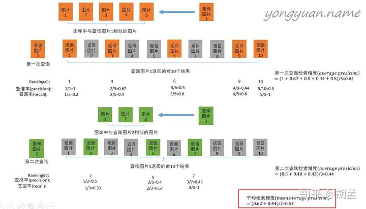
以上是图像检索中mAP的计算案例,简要说明下:
1 查询图片1在图像库中检索相似图像,假设图像库中有五张相似图像,表示为图片1、...、图片5,排名不分先后;
2 检索(过程略),返回了top-10图像,如上图第二行,橙色表示相似的图像,灰色为无关图像;
3 接下来就是precision、recall的计算过程了,结合上图比较容易理解;
以返回图片6的节点为例:
top-6中,有3张图像确实为相似图像,另三张图像为无关图像,因此precision = 3 / 6;同时,总共五张相似图像,top-6检索出来了三张,因此recall = 3 / 5;
4 然后计算AP,可以看右边的计算方式,可以发现是把列出来的查询率(precision)相加取平均,那么最关键的问题来了:为什么选择这几张图像的precision求平均?可惜图中并没有告诉我们原因;
但其实不难,一句话就是:选择每个recall区间内对应的最高precision;
举个栗子,以上图橙色检索案例为例,当我们只选择top-1作为检索结果返回(也即只返回一个检索结果)时,检索性能为:
top-1:recall = 1 / 5、precision = 1 / 1;# 以下类推;
top-2:recall = 1 / 5、precision = 1 / 2;
top-3:recall = 2 / 5、precision = 2 / 3;
top-4:recall = 2 / 5、precision = 2 / 4;
top-5:recall = 2 / 5、precision = 2 / 5;
top-6:recall = 3 / 5、precision = 3 / 6;
top-7:recall = 3 / 5、precision = 3 / 7;
top-8:recall = 3 / 5、precision = 3 / 8;
top-9:recall = 4 / 5、precision = 4 / 9;
top-10:recall = 5 / 5、precision = 5 / 10;
结合上面清单,先找找recall = 1 / 5区间下的最高precision,对应着precision = 1 / 1;
同理,recall = 2 / 5区间下的最高precision,对应着precision = 2 / 3;
recall = 3 / 5区间下的最高precision,对应着precision = 3 / 6;依次类推;
这样AP = (1 / 1 + 2 / 3 + 3 / 6 + 4 / 9 + 5 / 10) / 5;
那么mAP是啥?计算所有检索图像返回的AP均值,对应上图就是橙、绿突图像计算AP求均值,对应红色框;
这样mAP就计算完毕啦~~~是不是很容易理解?目标检测的mAP也是类似操作了;
2 目标检测中mAP计算流程
这里面我引用的是一篇博文,以下内容大多参考该博文,做了一些小修改;
下面的例子也很容易理解,假设检测人脸吧,gt label表示1为人脸,0为bg,某张图像中共检出了20个pred bbox,id:1 ~ 20,并对应了confidence score,gt label也很容易获得,pred bbox与gt bbox算IoU,给定一个threshold,那么就知道该pred bbox是否为正确的预测结果了,就对应了其gt label;---- 其实下表不应该这么理解的,但我们还是先这么认为,忽略差异吧,先直捣黄龙,table 1:
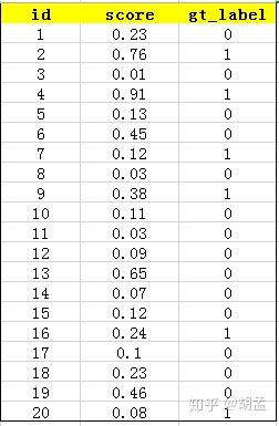
接下来对confidence score排序,得到table 2:
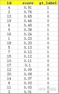
这张表很重要,接下来的precision和recall都是依照这个表计算的,那么这里的confidence score其实就和图像检索中的相似度关联上了,具体地,就是如第一节的图像检索中,虽然我们计算mAP没在乎其检索返回的先后顺序,但top1肯定是与待检索图像最相似的,对应的similarity score最高,对人脸检测而言,pred bbox的confidence score最高,也说明该bbox最有可能是人脸;
然后计算precision和recall,这两个标准的定义如下:
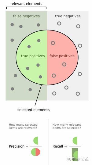
上面的图看看就行,能理解就理解,不理解可以参照第一节图像检索的例子来理解;
现以返回的top-5结果为例,如table 3:
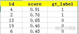
在这个例子中,true positives就是指id = 4、2的pred bbox,false positives就是指id = 13、19、6的pred bbox。方框内圆圈外的元素(false negatives + true negatives)是相对于方框内的元素而言,在这个例子中,是指confidence score排在top-5之外的元素,即table 4:
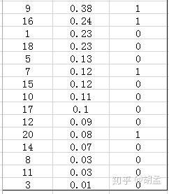
其中,false negatives是指id = 9、16、7、20的4个pred bbox,true negatives是指id = 1、18、5、15、10、17、12、14、8、11、3的11个pred bbox;
那么,这个例子中Precision = 2 / 5 = 40%,意思是对于人脸检测而言,我们选定了5 pred bbox,其中正确的有2个,即准确率为40%;Recall = 2 / 6 = 33%,意思是该图像中共有6个人脸,但是因为我们只召回了2个,所以召回率为33%;
实际的目标检测任务中,我们通常不满足只通过top-5来衡量一个模型的好坏,而是需要知道从top-1到top-N(N是所有pred bbox,本文中为20)对应的precision和recall;显然随着我们选定的pred bbox越来也多,recall一定会越来越高,而precision整体上会呈下降趋势;把recall当成横坐标,precision当成纵坐标,即可得到常用的precision-recall曲线,以上例子的precision-recall曲线如fig 1:
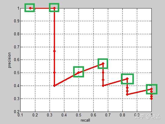
以上图像如何计算的?可以参照第一节图像检索中的栗子,还是比较容易理解的吧;
上面的每个红点,就相当于根据table 2,按照第一节中图像检索的方式计算出来的,也可以直接参照下面的table 5,自己心里算一算;
那么按照选择每个recall区间内对应的最高precision的计算方案,各个recall区间内对应的top-precision,就刚好如fig 1中的绿色框位置,可以进一步结合table 5中的绿色框理解;
好了,那么对这张图像而言,其AP = (1 / 1 + 2 / 2 + 3 / 6 + 4 / 7 + 5 / 11 + 6 / 16)/ 6;这是针对单张图像而言,所有图像也类似方式计算,那么就可以根据所有图像上的pred bbox,采用同样的方式,就计算出了所有图像上人脸这个类的AP;因为人脸检测只有一个类,如Pascal VOC这种20类的,每类都可以计算出一个AP,那么AP_total / 20,就是mAP啦;
但是等等,有没有发现table 5中,计算方式好像跟我们讲的有一点不一样?我们继续看看;
3 Pascal VOC的两套mAP评估标准
Pascal VOC中对mAP的计算经历了两次迭代,一种是VOC07的计算标准,对应绿色框:
首先设定一组阈值,T = [0、0.1、0.2、…、1],然后对于recall大于每一个阈值Ti(比如recall > 0.3),我们都会在该recall区间内得到一个对应的最大precision,这样我们就计算出了11个precision;----- 这里与上两节介绍的概念是一样的,只不过上面recall的区间是参照gt label来划分的,这里是我们人为划分的11个节点;
AP即为这11个precision的平均值,这种方法英文叫做11-point interpolated average precision;有了一个类的AP,所有类的AP均值即为mAP;
另一种是VOC10的计算标准,对应白色框:
新的计算方法假设N个pred bbox中有M个gt bbox,那么我们会得到M个recall节点(1 / M、2 / M、...、 M / M),对于每个recall值 r,我们可以计算出对应(r' > r)的最大precision,然后对这M个precision值取平均即得到最后的AP值,计算方法如table 5:
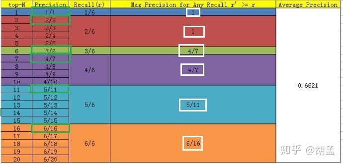
从VOC07的绿框、VOC10的白框对比可知,差异主要在recall = 3 / 6下的precision,可以发现VOC07找的top-precision是在该recall区间段内的,但VOC10相当于是向后查找的,需确保该recall阈值以后的区间内,对应的是top-precision,可知4 / 7 > 3 / 6,因此使用4 / 7替换了3 / 6,其他recall阈值下的操作方式类似;
那么代码的实操中,就得从按照recall阈值从后往前计算了,这样就可以一遍就梭哈出所有结果,如果按recall从前往后计算,就有很多重复性计算(不断地重复向后recall区间内查找top-precision),然后呢,就可以使用到动态规划的方式做了,理论结合实践啊有木有~~~
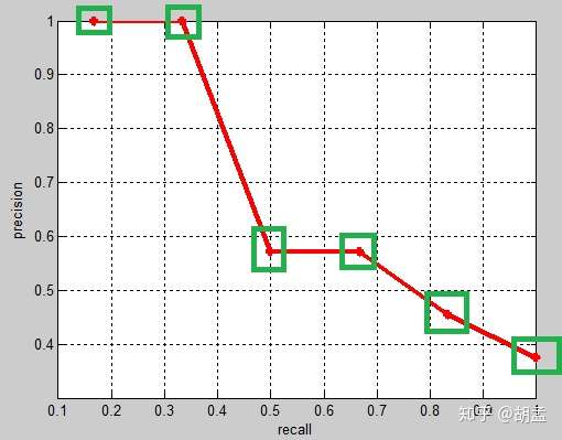
那么VOC10下,相应的Precision-Recall曲线如fig 2,可以发现这条曲线是单调递减的,剩下的AP计算方式就与VOC07相同了:
这里还需要继续一点,VOC07是11点插值的AP方式,等于是卡了11个离散的点,划分10个区间来计算AP,但VOC10是是根据recall值变化的区间来计算的,在这个栗子里,recall只变化了6次,但如果recall变化很多次,如100次、1000次、9999次等,就可以认为是一种 “伪” 连续的方式计算了;
总结:
AP衡量的是模型在每个类别上的好坏,mAP衡量的是模型在所有类别上的好坏,得到AP后mAP的计算就变得很简单了,就是取所有类别AP的平均值。
3 代码
直接上代码吧,这个函数假设我们已经得到了排序好的precision、recall的list,对应上图fig 2,进一步可以参照第一节中的清单理解;
# VOC-style mAP,分为两个计算方式,之所有两个计算方式,是因为2010年后VOC更新了评估方法,因此就有了07-metric和else...
def voc_ap(rec, prec, use_07_metric=False):
    """
    average precision calculations
    [precision integrated to recall]
    :param rec: recall list
    :param prec: precision list
    :param use_07_metric: 2007 metric is 11-recall-point based AP
    :return: average precision
    """
    if use_07_metric:
        # 11 point metric
        ap = 0.
        # VOC07是11点插值的AP方式,等于是卡了11个离散的点,划分10个区间来计算AP
        for t in np.arange(0., 1.1, 0.1):
            if np.sum(rec >= t) == 0:
                p = 0    # recall卡的阈值到顶了,1.1
            else:
                p = np.max(prec[rec >= t])   # VOC07:选择每个recall区间内对应的最高precision的计算方案
            ap = ap + p / 11.    # 11-recall-point based AP
    else:
        # correct AP calculation
        # first append sentinel values at the end
        mrec = np.concatenate(([0.], rec, [1.]))
        mpre = np.concatenate(([0.], prec, [0.]))

        # compute the precision envelope
        for i in range(mpre.size - 1, 0, -1):
            mpre[i - 1] = np.maximum(mpre[i - 1], mpre[i])    # 这个是不是动态规划?从后往前找之前区间内的top-precision,多么优雅的代码呀~~~

        # to calculate area under PR curve, look for points where X axis (recall) changes value
        # 上面的英文,可以结合着fig 2的绿框理解,一目了然
        # VOC10是是根据recall值变化的区间来计算的,如果recall变化很多次,就可以认为是一种 “伪” 连续的方式计算了,以下求的是recall的变化
        i = np.where(mrec[1:] != mrec[:-1])[0]

        # 计算AP,这个计算方式有点玄乎,是一个积分公式的简化,应该是对应的fig 2中红色曲线以下的面积,之前公式的推导我有看过,现在有点忘了,麻烦各位同学补充一下
        # 现在理解了,不难,公式:sum (\Delta recall) * prec,其实结合fig2和下面的图,不就是算的积分么?如果recall划分得足够细,就可以当做连续数据,然后以下公式就是积分公式,算的precision、recall下面的面积了
        ap = np.sum((mrec[i + 1] - mrec[i]) * mpre[i + 1])
    return ap
通常VOC10标准下计算的mAP值会高于VOC07,原因如下,我就不详细介绍了:
Interpolated average precision Some authors choose an alternate approximation that is called the interpolated average precision. Often, they still call it average precision. Instead of using P(k), the precision at a retrieval cutoff of k images, the interpolated average precision uses:

In other words, instead of using the precision that was actually observed at cutoff k, the interpolated average precision uses the maximum precision observed across all cutoffs with higher recall. The full equation for computing the interpolated average precision is:
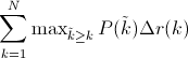
Visually, here’s how the interpolated average precision compares to the approximated average precision (to show a more interesting plot, this one isn’t from the earlier example):
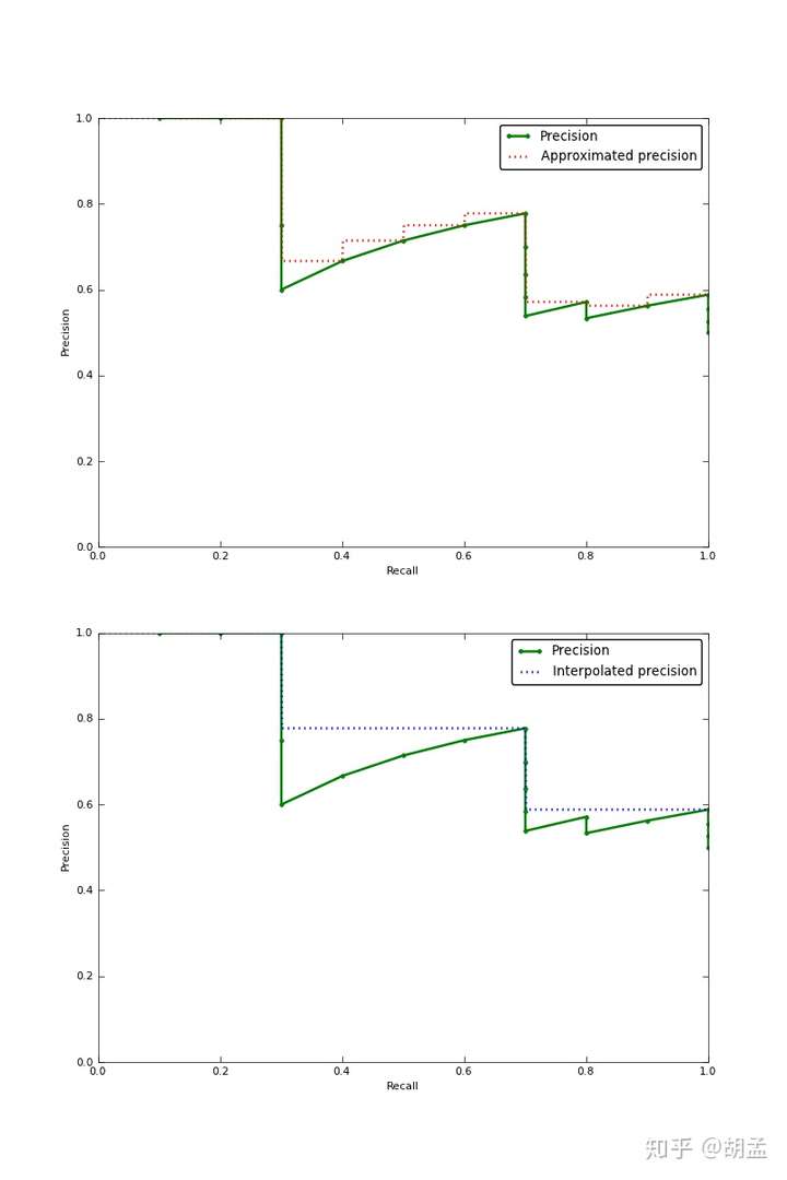
The approximated average precision closely hugs the actually observed curve. The interpolated average precision over estimates the precision at many points and produces a higher average precision value than the approximated average precision.
Further, there are variations on where to take the samples when computing the interpolated average precision. Some take samples at a fixed 11 points from 0 to 1: {0, 0.1, 0.2, …, 0.9, 1.0}. This is called the 11-point interpolated average precision. Others sample at every k where the recall changes.
参考资料
- TODO
参考资料
- https://github.com/Cartucho/mAP
- https://github.com/rafaelpadilla/Object-Detection-Metrics
- 【目标检测】VOC mAP
-
mAP
-
FPS
-
TODO
参考资料
- TODO
- PA
- MP
- mIoU
- FWIoU
参考资料
- 《A Review on Deep Learning Techniques Applied to Semantic Segmentation》
- 图像语义分割准确率度量方法总结
- 论文笔记 | 基于深度学习的图像语义分割技术概述之5.1度量标准
- TODO
- [ ]
参考资料
- TODO
参考资料
- [ ]
参考资料
- TODO
- TODO
- TODO
- TODO
- TODO
- TODO
多尺度训练对全卷积网络有效,一般设置几种不同尺度的图片,训练时每隔一定iterations随机选取一种尺度训练。这样训练出来的模型鲁棒性强,其可以接受任意大小的图片作为输入,使用尺度小的图片测试速度会快些,但准确度低,用尺度大的图片测试速度慢,但是准确度高。
参考资料
参考资料
- 样本贡献不均:Focal Loss和 Gradient Harmonizing Mechanism
- 被忽略的Focal Loss变种
- Soft Sampling:探索更有效的采样策略:介绍了Focal Loss、GHM和PISA
- TODO
参考资料
- TODO
- TODO
- TODO
参考资料
- TODO
参考资料
- TODO
参考资料
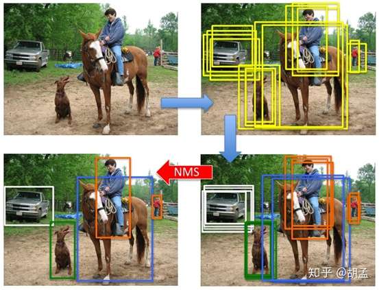
本笔记介绍目标检测的另一个基本概念:NMS(non-maximum suppression),做目标检测的同学想必对这个词语耳熟能详了;
在检测图像中的目标时,不可避免地会检出很多bboxes + cls scores,这些bbox之间有很多是冗余的,一个目标可能会被多个bboxes检出,如果所有bboxes都输出,就很影响体验和美观了(同一个目标输出100个bboxes,想想都后怕~~~),一种方案就是提升cls scores的阈值,减少bbox数量的输出;另一种方案就是使用NMS,将同一目标内的bboxes按照cls score + IoU阈值做筛选,剔除冗余地、低置信度的bbox;
可能又会问了:为什么目标检测时,会有这么多无效、冗余检测框呢?这个。。。我的理解,是因为图像中没有目标尺度、位置的先验知识,为保证对目标的高召回,就必须使用滑窗、anchor / default bbox密集采样的方式,尽管检测模型能对每个anchor / default bbox做出 cls + reg,可以一定程度上剔除误检,但没有结合检出bbox的cls score + IoU阈值做筛选,而NMS就可以做到这一点;
1 NMS操作流程
NMS用于剔除图像中检出的冗余bbox,标准NMS的具体做法为:
step-1:将所有检出的output_bbox按cls score划分(如pascal voc分20个类,也即将output_bbox按照其对应的cls score划分为21个集合,1个bg类,只不过bg类就没必要做NMS而已);
step-2:在每个集合内根据各个bbox的cls score做降序排列,得到一个降序的list_k;
step-3:从list_k中top1 cls score开始,计算该bbox_x与list中其他bbox_y的IoU,若IoU大于阈值T,则剔除该bbox_y,最终保留bbox_x,从list_k中取出;
step-4:选择list_k中top2 cls score(步骤3取出top 1 bbox_x后,原list_k中的top 2就相当于现list_k中的top 1了,但如果step-3中剔除的bbox_y刚好是原list_k中的top 2,就依次找top 3即可,理解这么个意思就行),重复step-3中的迭代操作,直至list_k中所有bbox都完成筛选;
step-5:对每个集合的list_k,重复step-3、4中的迭代操作,直至所有list_k都完成筛选;
以上操作写的有点绕,不过如果理解NMS操作流程的话,再结合下图,应该还是非常好理解的;
2 代码学习
2.1 test_RFB.py
我选择了RFBNet里的代码介绍NMS,因为里面的流程基本上就是按照我说的操作进行了;
先看看test_RFB.py中的片段,通过以下代码可以发现,其对应着step-1、step5操作,就是说NMS操作是逐类进行的,图像中检出的所有bboxes,按照 cls 做划分,再每个类的bbox进一步做NMS;
out = net(x)      # forward pass,这里相当于将图像 x 输入RFBNet,得到了pred cls + reg
boxes, scores = detector.forward(out,priors) # 结合priors,将pred reg(也即预测的offsets)解码成最终的pred bbox,如果理解anchor / default bbox操作流程,这个应该很好理解的;
boxes = boxes[0]
scores=scores[0]

# scale each detection back up to the image
boxes *= scale   # (0,1)区间坐标的bbox做尺度反正则化
boxes = boxes.cpu().numpy()
scores = scores.cpu().numpy()

for j in range(1, num_classes):      # 对每个类 j 的pred bbox单独做NMS,为什么index从1开始?因为0是bg,做NMS无意义
    inds = np.where(scores[:, j] > thresh)[0]     # 找到该类 j 下,所有cls score大于thresh的bbox,为什么选择大于thresh的bbox?因为score小于阈值的bbox,直接可以过滤掉,无需劳烦NMS
    if len(inds) == 0:    # 没有满足条件的bbox,返回空,跳过;
        all_boxes[j][i] = np.empty([0, 5], dtype=np.float32)
        continue
    c_bboxes = boxes[inds]
    c_scores = scores[inds, j]   # 找到对应类 j 下的score即可
    c_dets = np.hstack((c_bboxes, c_scores[:, np.newaxis])).astype(
        np.float32, copy=False)   # 将满足条件的bbox + cls score的bbox通过hstack完成合体

    keep = nms(c_dets, 0.45, force_cpu=args.cpu)    # NMS,返回需保存的bbox index:keep
    c_dets = c_dets[keep, :]
all_boxes[j][i] = c_dets # i 对应每张图像,j 对应图像中类别 j 的bbox清单介绍以上代码处理流程,两个目的:
1 test_RFB.py的处理流程非常清晰,也很方便我们的理解;
2 for j in range(1, num_classes)操作表明了,NMS是逐类进行的,也即参与NMS的bbox都属于同一类;
2.2 py_cpu_nms.py
代码同样来自于FRBNet,结合注释可以发现引自Fast R-CNN;
这个代码是最简版的nms,跟第一节中NMS处理流程一致,非常适合学习,可以作为baseline,我加了个简单的main函数做测试;
# --------------------------------------------------------
# Fast R-CNN
# Copyright (c) 2015 Microsoft
# Licensed under The MIT License [see LICENSE for details]
# Written by Ross Girshick
# --------------------------------------------------------

import numpy as np

def py_cpu_nms(dets, thresh):
    """Pure Python NMS baseline."""
    x1 = dets[:, 0]                     # pred bbox top_x
    y1 = dets[:, 1]                     # pred bbox top_y
    x2 = dets[:, 2]                     # pred bbox bottom_x
    y2 = dets[:, 3]                     # pred bbox bottom_y
    scores = dets[:, 4]              # pred bbox cls score

    areas = (x2 - x1 + 1) * (y2 - y1 + 1)    # pred bbox areas
    order = scores.argsort()[::-1]              # 对pred bbox按score做降序排序,对应step-2

    keep = []    # NMS后,保留的pred bbox
    while order.size > 0:
        i = order[0]          # top-1 score bbox
        keep.append(i)   # top-1 score的话,自然就保留了
        xx1 = np.maximum(x1[i], x1[order[1:]])   # top-1 bbox(score最大)与order中剩余bbox计算NMS
        yy1 = np.maximum(y1[i], y1[order[1:]])
        xx2 = np.minimum(x2[i], x2[order[1:]])
        yy2 = np.minimum(y2[i], y2[order[1:]])

        w = np.maximum(0.0, xx2 - xx1 + 1)
        h = np.maximum(0.0, yy2 - yy1 + 1)
        inter = w * h
        ovr = inter / (areas[i] + areas[order[1:]] - inter)      # 无处不在的IoU计算~~~

        inds = np.where(ovr <= thresh)[0]     # 这个操作可以对代码断点调试理解下,结合step-3,我们希望剔除所有与当前top-1 bbox IoU > thresh的冗余bbox,那么保留下来的bbox,自然就是ovr <= thresh的非冗余bbox,其inds保留下来,作进一步筛选
        order = order[inds + 1]   # 保留有效bbox,就是这轮NMS未被抑制掉的幸运儿,为什么 + 1?因为ind = 0就是这轮NMS的top-1,剩余有效bbox在IoU计算中与top-1做的计算,inds对应回原数组,自然要做 +1 的映射,接下来就是step-4的循环

    return keep    # 最终NMS结果返回

if __name__ == '__main__':
    dets = np.array([[100,120,170,200,0.98],
                     [20,40,80,90,0.99],
                     [20,38,82,88,0.96],
                     [200,380,282,488,0.9],
                     [19,38,75,91, 0.8]])

    py_cpu_nms(dets, 0.5)
2.2 bbox_utils.py
同样是RFBNet中的nms代码,用pytorch实现的,其实和2.1小节中的NMS操作完全一致;
# Original author: Francisco Massa:
# https://github.com/fmassa/object-detection.torch
# Ported to PyTorch by Max deGroot (02/01/2017)
def nms(boxes, scores, overlap=0.5, top_k=200):
    """Apply non-maximum suppression at test time to avoid detecting too many
    overlapping bounding boxes for a given object. ---- 这里面有一个细节,NMS仅用于测试阶段,为什么不用于训练阶段呢?可以评论留言下,我就不解释了,嘿嘿~~~
    Args:
        boxes: (tensor) The location preds for the img, Shape: [num_priors,4].
        scores: (tensor) The class predscores for the img, Shape:[num_priors].
        overlap: (float) The overlap thresh for suppressing unnecessary boxes.
        top_k: (int) The Maximum number of box preds to consider.
    Return:
        The indices of the kept boxes with respect to num_priors.
    """

    keep = torch.Tensor(scores.size(0)).fill_(0).long()
    if boxes.numel() == 0:
        return keep
    x1 = boxes[:, 0]
    y1 = boxes[:, 1]
    x2 = boxes[:, 2]
    y2 = boxes[:, 3]
    area = torch.mul(x2 - x1, y2 - y1)    # IoU初步准备
    v, idx = scores.sort(0)  # sort in ascending order,对应step-2,不过是升序操作,非降序
    # I = I[v >= 0.01]
    idx = idx[-top_k:]  # indices of the top-k largest vals,依然是升序的结果
    xx1 = boxes.new()
    yy1 = boxes.new()
    xx2 = boxes.new()
    yy2 = boxes.new()
    w = boxes.new()
    h = boxes.new()

    # keep = torch.Tensor()
    count = 0
    while idx.numel() > 0:   # 对应step-4,若所有pred bbox都处理完毕,就可以结束循环啦~
        i = idx[-1]  # index of current largest val,top-1 score box,因为是升序的,所有返回index = -1的最后一个元素即可
        # keep.append(i)
        keep[count] = i
        count += 1    # 不仅记数NMS保留的bbox个数,也作为index存储bbox
        if idx.size(0) == 1:
            break
        idx = idx[:-1]  # remove kept element from view,top-1已保存,不需要了~~~
        # load bboxes of next highest vals
        torch.index_select(x1, 0, idx, out=xx1)
        torch.index_select(y1, 0, idx, out=yy1)
        torch.index_select(x2, 0, idx, out=xx2)
        torch.index_select(y2, 0, idx, out=yy2)
        # store element-wise max with next highest score
        xx1 = torch.clamp(xx1, min=x1[i])   # 对应 np.maximum(x1[i], x1[order[1:]])
        yy1 = torch.clamp(yy1, min=y1[i])
        xx2 = torch.clamp(xx2, max=x2[i])
        yy2 = torch.clamp(yy2, max=y2[i])
        w.resize_as_(xx2)
        h.resize_as_(yy2)
        w = xx2 - xx1
        h = yy2 - yy1
        # check sizes of xx1 and xx2.. after each iteration
        w = torch.clamp(w, min=0.0)    # clamp函数可以去查查,类似max、mini的操作
        h = torch.clamp(h, min=0.0)
        inter = w*h
        # IoU = i / (area(a) + area(b) - i)
        # 以下两步操作做了个优化,area已经计算好了,就可以直接根据idx读取结果了,area[i]同理,避免了不必要的冗余计算
        rem_areas = torch.index_select(area, 0, idx)  # load remaining areas)
        union = (rem_areas - inter) + area[i]     # 就是area(a) + area(b) - i
        IoU = inter/union  # store result in iou,# IoU来啦~~~
        # keep only elements with an IoU <= overlap
        idx = idx[IoU.le(overlap)]   # 这一轮NMS操作,IoU阈值小于overlap的idx,就是需要保留的bbox,其他的就直接忽略吧,并进行下一轮计算
    return keep, count
2.2 cpu_nms.pyx
同样在RGBNet项目中,下面就是优化后的NNS操作,以及soft-NMS操作,我就不细讲了~~~
# --------------------------------------------------------
# Fast R-CNN
# Copyright (c) 2015 Microsoft
# Licensed under The MIT License [see LICENSE for details]
# Written by Ross Girshick
# --------------------------------------------------------

import numpy as np
cimport numpy as np

cdef inline np.float32_t max(np.float32_t a, np.float32_t b):
    return a if a >= b else b

cdef inline np.float32_t min(np.float32_t a, np.float32_t b):
    return a if a <= b else b

def cpu_nms(np.ndarray[np.float32_t, ndim=2] dets, np.float thresh):
    cdef np.ndarray[np.float32_t, ndim=1] x1 = dets[:, 0]
    cdef np.ndarray[np.float32_t, ndim=1] y1 = dets[:, 1]
    cdef np.ndarray[np.float32_t, ndim=1] x2 = dets[:, 2]
    cdef np.ndarray[np.float32_t, ndim=1] y2 = dets[:, 3]
    cdef np.ndarray[np.float32_t, ndim=1] scores = dets[:, 4]

    cdef np.ndarray[np.float32_t, ndim=1] areas = (x2 - x1 + 1) * (y2 - y1 + 1)
    cdef np.ndarray[np.int_t, ndim=1] order = scores.argsort()[::-1]

    cdef int ndets = dets.shape[0]
    cdef np.ndarray[np.int_t, ndim=1] suppressed = \
            np.zeros((ndets), dtype=np.int)

    # nominal indices
    cdef int _i, _j
    # sorted indices
    cdef int i, j
    # temp variables for box i's (the box currently under consideration)
    cdef np.float32_t ix1, iy1, ix2, iy2, iarea
    # variables for computing overlap with box j (lower scoring box)
    cdef np.float32_t xx1, yy1, xx2, yy2
    cdef np.float32_t w, h
    cdef np.float32_t inter, ovr

    keep = []
    for _i in range(ndets):
        i = order[_i]
        if suppressed[i] == 1:
            continue
        keep.append(i)
        ix1 = x1[i]
        iy1 = y1[i]
        ix2 = x2[i]
        iy2 = y2[i]
        iarea = areas[i]
        for _j in range(_i + 1, ndets):
            j = order[_j]
            if suppressed[j] == 1:
                continue
            xx1 = max(ix1, x1[j])
            yy1 = max(iy1, y1[j])
            xx2 = min(ix2, x2[j])
            yy2 = min(iy2, y2[j])
            w = max(0.0, xx2 - xx1 + 1)
            h = max(0.0, yy2 - yy1 + 1)
            inter = w * h
            ovr = inter / (iarea + areas[j] - inter)
            if ovr >= thresh:
                suppressed[j] = 1

    return keep

def cpu_soft_nms(np.ndarray[float, ndim=2] boxes, float sigma=0.5, float Nt=0.3, float threshold=0.001, unsigned int method=0):
    cdef unsigned int N = boxes.shape[0]
    cdef float iw, ih, box_area
    cdef float ua
    cdef int pos = 0
    cdef float maxscore = 0
    cdef int maxpos = 0
    cdef float x1,x2,y1,y2,tx1,tx2,ty1,ty2,ts,area,weight,ov

    for i in range(N):
        maxscore = boxes[i, 4]
        maxpos = i

        tx1 = boxes[i,0]
        ty1 = boxes[i,1]
        tx2 = boxes[i,2]
        ty2 = boxes[i,3]
        ts = boxes[i,4]

        pos = i + 1
	# get max box
        while pos < N:
            if maxscore < boxes[pos, 4]:
                maxscore = boxes[pos, 4]
                maxpos = pos
            pos = pos + 1

	# add max box as a detection
        boxes[i,0] = boxes[maxpos,0]
        boxes[i,1] = boxes[maxpos,1]
        boxes[i,2] = boxes[maxpos,2]
        boxes[i,3] = boxes[maxpos,3]
        boxes[i,4] = boxes[maxpos,4]

	# swap ith box with position of max box
        boxes[maxpos,0] = tx1
        boxes[maxpos,1] = ty1
        boxes[maxpos,2] = tx2
        boxes[maxpos,3] = ty2
        boxes[maxpos,4] = ts

        tx1 = boxes[i,0]
        ty1 = boxes[i,1]
        tx2 = boxes[i,2]
        ty2 = boxes[i,3]
        ts = boxes[i,4]

        pos = i + 1
	# NMS iterations, note that N changes if detection boxes fall below threshold
        while pos < N:
            x1 = boxes[pos, 0]
            y1 = boxes[pos, 1]
            x2 = boxes[pos, 2]
            y2 = boxes[pos, 3]
            s = boxes[pos, 4]

            area = (x2 - x1 + 1) * (y2 - y1 + 1)
            iw = (min(tx2, x2) - max(tx1, x1) + 1)
            if iw > 0:
                ih = (min(ty2, y2) - max(ty1, y1) + 1)
                if ih > 0:
                    ua = float((tx2 - tx1 + 1) * (ty2 - ty1 + 1) + area - iw * ih)
                    ov = iw * ih / ua #iou between max box and detection box

                    if method == 1: # linear
                        if ov > Nt:
                            weight = 1 - ov
                        else:
                            weight = 1
                    elif method == 2: # gaussian
                        weight = np.exp(-(ov * ov)/sigma)
                    else: # original NMS
                        if ov > Nt:
                            weight = 0
                        else:
                            weight = 1

                    boxes[pos, 4] = weight*boxes[pos, 4]

		    # if box score falls below threshold, discard the box by swapping with last box
		    # update N
                    if boxes[pos, 4] < threshold:
                        boxes[pos,0] = boxes[N-1, 0]
                        boxes[pos,1] = boxes[N-1, 1]
                        boxes[pos,2] = boxes[N-1, 2]
                        boxes[pos,3] = boxes[N-1, 3]
                        boxes[pos,4] = boxes[N-1, 4]
                        N = N - 1
                        pos = pos - 1

            pos = pos + 1

    keep = [i for i in range(N)]
    return keep
参考代码:
https://github.com/ruinmessi/RFBNet:RFBNet
https://github.com/rbgirshick/py-faster-rcnn:学习一百遍都不为过的faster rcnn
NMS_demo.py:https://github.com/humengdoudou/object_detection_mAP/blob/master/NMS_demo.py
参考资料
-
NMS
-
Soft-NMS
-
Softer-NMS
-
IoU-guided NMS
-
ConvNMS
-
Pure NMS
-
Yes-Net
-
LNMS
-
INMS
-
Polygon NMS
-
MNMS
参考资料
- TODO
- TODO
- TODO
- TODO
RPN结构说明:
-
从基础网络提取的第五卷积层特征进入RPN后分为两个分支,其中一个分支进行针对feature map(上图conv-5-3共有512个feature-map)的每一个位置预测共(9*4=36)个参数,其中9代表的是每一个位置预设的9种形状的anchor-box,4对应的是每一个anchor-box的预测值(该预测值表示的是预设anchor-box到ground-truth-box之间的变换参数),上图中指向rpn-bbox-pred层的箭头上面的数字36即是代表了上述的36个参数,所以rpn-bbox-pred层的feature-map数量是36,而每一张feature-map的形状(大小)实际上跟conv5-3一模一样的;
-
另一分支预测该anchor-box所框定的区域属于前景和背景的概率(网上很对博客说的是,指代该点属于前景背景的概率,那样是不对的,不然怎么会有18个feature-map输出呢?否则2个就足够了),前景背景的真值给定是根据当前像素(anchor-box中心)是否在ground-truth-box内;
-
上图RPN-data(python)运算框内所进行的操作是读取图像信息(原始宽高),groun-truth boxes的信息(bounding-box的位置,形状,类别)等,作好相应的转换,输入到下面的层当中。
-
要注意的是RPN内部有两个loss层,一个是BBox的loss,该loss通过减小ground-truth-box与预测的anchor-box之间的差异来进行参数学习,从而使RPN网络中的权重能够学习到预测box的能力。实现细节是每一个位置的anchor-box与ground-truth里面的box进行比较,选择IOU最大的一个作为该anchor-box的真值,若没有,则将之class设为背景(概率值0,否则1),这样背景的anchor-box的损失函数中每个box乘以其class的概率后就不会对bbox的损失函数造成影响。另一个loss是class-loss,该处的loss是指代的前景背景并不是实际的框中物体类别,它的存在可以使得在最后生成roi时能快速过滤掉预测值是背景的box。也可实现bbox的预测函数不受影响,使得anchor-box能(专注于)正确的学习前景框的预测,正如前所述。所以,综合来讲,整个RPN的作用就是替代了以前的selective-search方法,因为网络内的运算都是可GPU加速的,所以一下子提升了ROI生成的速度。可以将RPN理解为一个预测前景背景,并将前景框定的一个网络,并进行单独的训练,实际上论文里面就有一个分阶段训练的训练策略,实际上就是这个原因。
-
最后经过非极大值抑制,RPN层产生的输出是一系列的ROI-data,它通过ROI的相对映射关系,将conv5-3中的特征已经存入ROI-data中,以供后面的分类网使用。
另外两个loss层的说明: 也许你注意到了,最后还有两个loss层,这里的class-loss指代的不再是前景背景loss,而是真正的类别loss了,这个应该就很好理解了。而bbox-loss则是因为rpn提取的只是前景背景的预测,往往很粗糙,这里其实是通过ROI-pooling后加上两层全连接实现更精细的box修正(这里其实是我猜的)。 ROI-Pooing的作用是为了将不同大小的Roi映射(重采样)成统一的大小输入到全连接层去。
以上。
参考资料
- TODO
参考资料
- TODO
- TODO
- TODO
参考资料
- TODO
- TODO
- TODO
- TODO
- TODO
- TODO
参考资料
《Focal Loss for Dense Object Detection》
清华大学孔涛博士在知乎上这么写道:
目标的检测和定位中一个很困难的问题是,如何从数以万计的候选窗口中挑选包含目标物的物体。只有候选窗口足够多,才能保证模型的 Recall。
目前,目标检测框架主要有两种:
一种是 one-stage ,例如 YOLO、SSD 等,这一类方法速度很快,但识别精度没有 two-stage 的高,其中一个很重要的原因是,利用一个分类器很难既把负样本抑制掉,又把目标分类好。
另外一种目标检测框架是 two-stage ,以 Faster RCNN 为代表,这一类方法识别准确度和定位精度都很高,但存在着计算效率低,资源占用大的问题。
Focal Loss 从优化函数的角度上来解决这个问题,实验结果非常 solid,很赞的工作。
何恺明团队提出了用 Focal Loss 函数来训练。
因为,他在训练过程中发现,类别失衡是影响 one-stage 检测器准确度的主要原因。那么,如果能将“类别失衡”这个因素解决掉,one-stage 不就能达到比较高的识别精度了吗?
于是在研究中,何恺明团队采用 Focal Loss 函数来消除“类别失衡”这个主要障碍。
结果怎样呢?
为了评估该损失的有效性,该团队设计并训练了一个简单的密集目标检测器—RetinaNet。试验结果证明,当使用 Focal Loss 训练时,RetinaNet 不仅能赶上 one-stage 检测器的检测速度,而且还在准确度上超越了当前所有最先进的 two-stage 检测器。
参考
- TODO
参考资料
- TODO
参考资料
参考资料
CornerNet介绍
- TODO
参考资料
- 目标检测方向
- 图像分割方向
- 目标跟踪方向
- 人脸(检测&识别&关键点)
- OCR方向
- SLAM方向
- 超分辨率
- 医疗影响方向
- Re-ID