This seminar was developed by Keegan Korthauer from materials previously designed by Eric Chu, Dr. Jenny Bryan, and Alice Zhu.
By the end of this seminar, you should
- have a clear understanding of what differential expression is and how it can be tested
- have practical experience browsing and manipulating real gene expression data
- have practical experience plotting expression changes as a trajectory using ggplot2
- have practical experience testing for differential expression in a
single gene using
lm() - have practical experience finding differential expressions in a large
number of genes and across multiple covariates using
limma() - have an intuition of how limma works in the context of “moderated” t-values
- be able to perform genome wide differential expression analysis given expression data and covariates and interpret the resulting statistics
We first load the packages we will use. We have previousy used knitr,
tidyverse and GEOquery. Today, we will also use
limma.
-
If you don’t have it already, first install the Bioconductor package manager package:
install.packages("BiocManager") -
Then install limma with
BiocManager::install("limma")
library(knitr)
library(tidyverse)
library(GEOquery)
library(limma)utils::read.table()- Reads a file in table format and creates a dataframe from it.base::c()- Combine arguments into a single data structure; for example, c(1,2,3) -> a vector containing 1, 2, and 3.base::names()- Functions to get or set the names of an object (vector, tibble, data frame, etc).base::factor()- The function factor is used to encode a vector as a factor.base::ncol()- Get the number of columns in a dataframe.base::nrow()- Get the number of rows in a dataframe.base::sort()- Sort a vector into ascending or descending order.tibble::rownames_to_column()- Opposite tocolumn_to_rownames(); convert row names to a column inside a dataframe.tibble::column_to_rownames()- Opposite torownames_to_column(); convert a column into a dataframe’s row names.tibble::as_tibble()- Convert a dataframe to a tibble.dplyr::pivot_longer()- Reduces the number of columns by moving values from all columns to one value per row, lengthening the data dimensions.base::t()- Transpose a matrix or dataframe.stats::t.test()- Performs one and two sample t-tests on vectors of data.stats::lm()- Fit linear models.base::summary()- Generic function used to produce result summaries of the results of various model fitting functions.stats::aov()- Fit an analysis of variance model by a call to lm for each stratum.knitr::kable()- Table generator for R-Markdown.base::all()- Given a set of logical vectors, are all of the values true?stats::model.matrix()- Creates a design (or model) matrix, e.g., by expanding factors to a set of summary variables.limma::lmFit()- Fit linear model for each gene given a series of arrays.limma::eBayes()- Empirical Bayes Statistics for Differential Expression.limma::topTable()- Extract a table of the top-ranked genes from a linear model fit.limma::makeContrasts()- Construct the contrast matrix corresponding to specified contrasts of a set of parameters.limma::contrast.fit()- Given a linear model fit to microarray data, compute estimated coefficients and standard errors for a given set of contrasts.limma::decideTests()- Identify which genes are significantly differentially expressed for each contrast from a fit object containing p-values and test statistics.base::intersect()- Set intersection.base::as.character()- Coerce object to character type, e.g. convert a factor into character.utils::head()- Return first part of a object (a vector or dataframe).
If the idea of differential gene expression sounds completely strange, make sure to review the relevant lecture notes and slides before you start. But, just briefly, for our purpose, the expression of a gene is simply the amount of its mRNA molecule that has been detected; the higher the abundance of mRNA detected, the higher the expression. And as with most other scientists, bioinformaticians are also interested in measuring differences between conditions. So, we’d like to know if genes are differentially expressed across ‘conditions’: e.g. healthy vs. disease, young vs. old, treatment vs. control, heart tissue vs skeletal muscle tissue, etc. And we have an elaborate statistical framework that helps us make this assessment.
Specifically, we may take a single gene and assess whether it is differentially expressed across some conditions. Or we may perform differential expression analysis on a large set of genes (sometimes all ~20,000 genes in the human genome) and do a high throughput screen to detect differentially expressed genes across some conditions. In this seminar, we will work through both scenarios. The approaches are fundamentally the same, but are also quite different, as you will soon see.
First, we introduce the gene expression dataset: its usual format &
organization. We will import a sample dataset and render a few plots and
tables to get you oriented. Next, we perform differential expression
analysis on a single gene. This will be important for understanding the
fundamental approach for assessing differential expression. Finally, we
perform a genome wide differential expression screen using limma (a
popular R package).
So, what does gene expression data look like?
In this seminar, we will use the GSE4051 dataset. See here for more details about the dataset. This is the same data set we’ve been exploring in class!
First we import the dataset. Note that we could read in the individual
expression data table and meta data table separately, but we’ll make use
of what we learned in last seminar, and obtain this data directly from
GEO using the GEOquery package. When fetching a “GSE” accession, the
getGEO function will return a list of ExpressionSet objects (more on
that in a bit), so we’ll use [[1]] notation to grab the first (and
only) element of that list.
eset <- getGEO("GSE4051", getGPL = FALSE)[[1]]## Found 1 file(s)
## GSE4051_series_matrix.txt.gz
eset## ExpressionSet (storageMode: lockedEnvironment)
## assayData: 45101 features, 39 samples
## element names: exprs
## protocolData: none
## phenoData
## sampleNames: GSM92610 GSM92611 ... GSM92648 (39 total)
## varLabels: title geo_accession ... relation (36 total)
## varMetadata: labelDescription
## featureData: none
## experimentData: use 'experimentData(object)'
## pubMedIds: 16505381
## Annotation: GPL1261
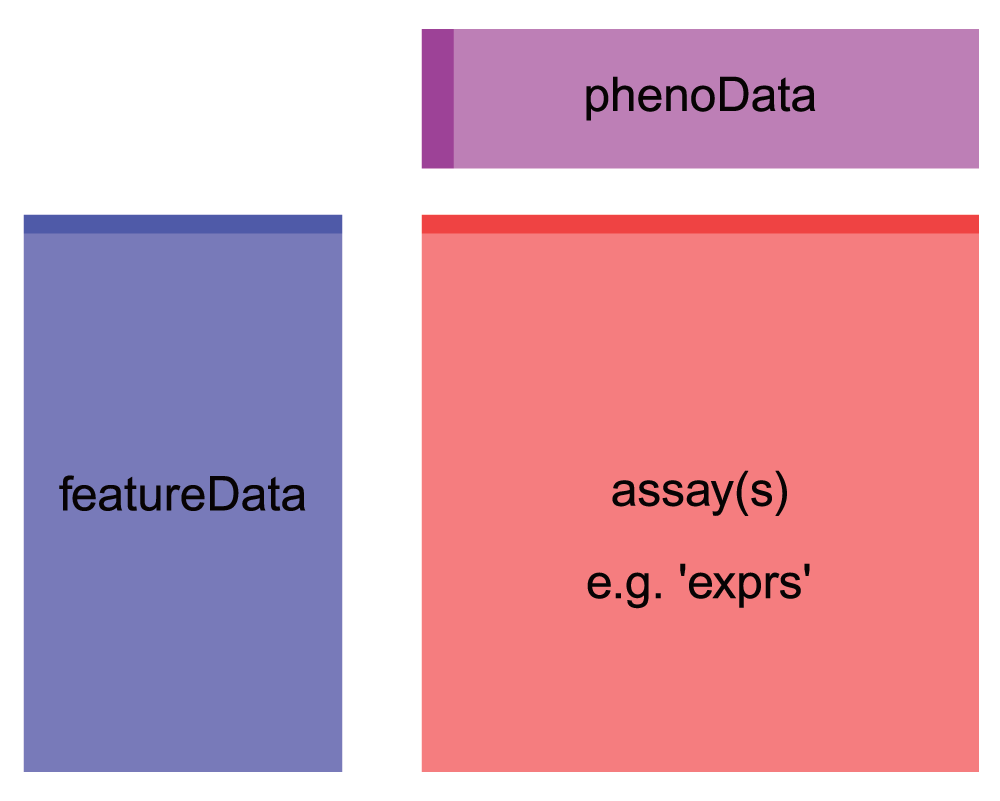
First, we notice that the object we get out is a specially formatted
object of class ExpressionSet. It has slots for the assay (expression)
data (assayData), and sample metadata (phenoData). We also have some
feature (gene) metadata in a slot called featureData. Note that this
object format is very similar to the SummarizedExperiment objects we
learned about in class - so this data is organized the Bioconductor way,
with all data housed in one object (that we are calling eset). Note
that we could convert this directly into a SummarizedExperiment object
by calling SummarizedExperiment(eset). But we’ll stick with this
format since it will serve our purposes just fine.
Let’s take a peek at what’s in the expression matrix, which we can
access from the ExpressionSet object with exprs(). It contains the
sample IDs and their corresponding gene expression profiles.
Essentially, each column is a different sample (a tissue, under some
treatment, during some developmental stage, etc) and each row is a gene
(or a probe). The expression values for all of the genes in a single
column collectively constitute the gene expression profile of the sample
represented by that column.
Here, we’ll print out a small subset (first 5 rows and first 4 columns) of this matrix so you have an idea what it looks like. Note that the gene (probe) names are stored as rownames. The column names (starting with GSM) indicate Sample IDs.
exprs(eset)[1:5,1:4]## GSM92610 GSM92611 GSM92612 GSM92613
## 1415670_at 7.108863 7.322392 7.420947 7.351444
## 1415671_at 9.714002 9.797742 9.831072 9.658442
## 1415672_at 9.429030 9.846977 10.003092 9.914112
## 1415673_at 8.426974 8.404206 8.594600 8.404206
## 1415674_a_at 8.498338 8.458287 8.426651 8.372776
Now let’s explore the properties associated with each sample. For example, does sample GSM92610 belong to treatment or control? What developmental stage is it in? What tissue is it? How about sample GSM92611? GSM92612?
Without this information, the expression matrix is pretty much useless, at least for our purpose of assessing differential expression across conditions.
This information is stored in the samples metadata. Here we pull
that out of the ExpressionSet object and take a peek at it using the
pData() accessor function. We see that we have 36 variables for each
of our 39 samples. We’ll print the first 3 variables for the first 6
rows.
str(pData(eset))## 'data.frame': 39 obs. of 36 variables:
## $ title : chr "Nrl-ko-Gfp 4 weeks retina replicate 1" "Nrl-ko-Gfp 4 weeks replicate 2" "Nrl-ko-Gfp 4 weeks replicate 3" "Nrl-ko-Gfp 4 weeks replicate 4" ...
## $ geo_accession : chr "GSM92610" "GSM92611" "GSM92612" "GSM92613" ...
## $ status : chr "Public on Feb 28 2006" "Public on Feb 28 2006" "Public on Feb 28 2006" "Public on Feb 28 2006" ...
## $ submission_date : chr "Jan 16 2006" "Jan 16 2006" "Jan 16 2006" "Jan 16 2006" ...
## $ last_update_date : chr "Aug 28 2018" "Aug 28 2018" "Aug 28 2018" "Aug 28 2018" ...
## $ type : chr "RNA" "RNA" "RNA" "RNA" ...
## $ channel_count : chr "1" "1" "1" "1" ...
## $ source_name_ch1 : chr "Gfp purified cell" "purified Gfp+ photoreceptor cells" "Gfp+ photoreceptor cells" "Gfp+ photoreceptor cells" ...
## $ organism_ch1 : chr "Mus musculus" "Mus musculus" "Mus musculus" "Mus musculus" ...
## $ characteristics_ch1 : chr "Nrl-ko, purified Gfp+ photoreceptor cell" "Nrl-ko-Gfp, Gfp+ photoreceptor cells" "Nrl-ko-Gfp, Gfp+ photoreceptor cells" "Nrl-ko-Gfp, Gfp+ photoreceptor cells" ...
## $ molecule_ch1 : chr "total RNA" "total RNA" "total RNA" "total RNA" ...
## $ extract_protocol_ch1 : chr "mRNA was amplified using Nugene kit" "mRNA was amplified using Nugene kit" "mRNA was amplified using Nugene kit" "mRNA was amplified using Nugene kit" ...
## $ label_ch1 : chr "Biotin" "Biotin" "Biotin" "Biotin" ...
## $ label_protocol_ch1 : chr "Nugene kit protocol" "Nugene kit protocol" "Nugene kit protocol" "Nugene kit protocol" ...
## $ taxid_ch1 : chr "10090" "10090" "10090" "10090" ...
## $ hyb_protocol : chr "Affymetrix standard" "Affymetrix standard" "Affymetrix standard" "Affymetrix standard" ...
## $ scan_protocol : chr "Affymetrix standard" "Affymetrix standard" "Affymetrix standard" "Affymetrix standard" ...
## $ description : chr "Nrl-ko mice were mated with wt-Gfp mice in which Gfp expression is driven by Nrl promoter. Gfp+ photoreceptors "| __truncated__ "Nrl-ko mice were mated with wt-Gfp mice in which Gfp expression is driven by Nrl promoter. Gfp+ photoreceptors "| __truncated__ "Nrl-ko mice were mated with wt-Gfp mice in which Gfp expression is driven by Nrl promoter. Gfp+ photoreceptors "| __truncated__ "Nrl-ko mice were mated with wt-Gfp mice in which Gfp expression is driven by Nrl promoter. Gfp+ photoreceptors "| __truncated__ ...
## $ description.1 : chr "This is Nrl-ko-Gfp 4 weeks sample." "This is Nrl-ko-Gfp 4 weeks replicate 2" "This is Nrl-ko-Gfp 4 weeks replicate 3" "This is Nrl-ko-Gfp 4 weeks replicate 4." ...
## $ description.2 : chr "" "" "" "" ...
## $ data_processing : chr "RMA" "RMA" "RMA" "RMA" ...
## $ platform_id : chr "GPL1261" "GPL1261" "GPL1261" "GPL1261" ...
## $ contact_name : chr "Swaroop,,Anand" "Swaroop,,Anand" "Swaroop,,Anand" "Swaroop,,Anand" ...
## $ contact_email : chr "swaroop@umich.edu" "swaroop@umich.edu" "swaroop@umich.edu" "swaroop@umich.edu" ...
## $ contact_phone : chr "734-615 2246" "734-615 2246" "734-615 2246" "734-615 2246" ...
## $ contact_department : chr "Ophthalmology & Visual Sciences" "Ophthalmology & Visual Sciences" "Ophthalmology & Visual Sciences" "Ophthalmology & Visual Sciences" ...
## $ contact_institute : chr "University of Michigan" "University of Michigan" "University of Michigan" "University of Michigan" ...
## $ contact_address : chr "1000 Wall St." "1000 Wall St." "1000 Wall St." "1000 Wall St." ...
## $ contact_city : chr "Ann Arbor" "Ann Arbor" "Ann Arbor" "Ann Arbor" ...
## $ contact_state : chr "MI" "MI" "MI" "MI" ...
## $ contact_zip/postal_code: chr "48105" "48105" "48105" "48105" ...
## $ contact_country : chr "USA" "USA" "USA" "USA" ...
## $ contact_web_link : chr "http://www.umich.edu/~retina" "http://www.umich.edu/~retina" "http://www.umich.edu/~retina" "http://www.umich.edu/~retina" ...
## $ supplementary_file : chr "ftp://ftp.ncbi.nlm.nih.gov/geo/samples/GSM92nnn/GSM92610/suppl/GSM92610.CEL.gz" "ftp://ftp.ncbi.nlm.nih.gov/geo/samples/GSM92nnn/GSM92611/suppl/GSM92611.CEL.gz" "ftp://ftp.ncbi.nlm.nih.gov/geo/samples/GSM92nnn/GSM92612/suppl/GSM92612.CEL.gz" "ftp://ftp.ncbi.nlm.nih.gov/geo/samples/GSM92nnn/GSM92613/suppl/GSM92613.CEL.gz" ...
## $ data_row_count : chr "45101" "45101" "45101" "45101" ...
## $ relation : chr "Reanalyzed by: GSE119085" "Reanalyzed by: GSE119085" "Reanalyzed by: GSE119085" "Reanalyzed by: GSE119085" ...
head(pData(eset)[,1:3])## title geo_accession
## GSM92610 Nrl-ko-Gfp 4 weeks retina replicate 1 GSM92610
## GSM92611 Nrl-ko-Gfp 4 weeks replicate 2 GSM92611
## GSM92612 Nrl-ko-Gfp 4 weeks replicate 3 GSM92612
## GSM92613 Nrl-ko-Gfp 4 weeks replicate 4 GSM92613
## GSM92614 Nrl-ko-Gfp E16 replicate 1 GSM92614
## GSM92615 Nrl-ko-Gfp E16 replicate 2 GSM92615
## status
## GSM92610 Public on Feb 28 2006
## GSM92611 Public on Feb 28 2006
## GSM92612 Public on Feb 28 2006
## GSM92613 Public on Feb 28 2006
## GSM92614 Public on Feb 28 2006
## GSM92615 Public on Feb 28 2006
Notice that the developmental stage and genotype information are contained in the variable called ‘title’. In order to work with these as separate variables, we’ll need to do some data wrangling.
pData(eset) <- pData(eset) %>%
  mutate(sample_id = geo_accession) %>%
  mutate(dev_stage =  case_when(
    grepl("E16", title) ~ "E16",
    grepl("P2", title) ~ "P2",
    grepl("P6", title) ~ "P6",
    grepl("P10", title) ~ "P10",
    grepl("4 weeks", title) ~ "4_weeks"
  )) %>%
  mutate(genotype = case_when(
    grepl("Nrl-ko", title) ~ "NrlKO",
    grepl("wt", title) ~ "WT"
  ))

pData(eset) %>%
  with(table(dev_stage, genotype))
## genotype
## dev_stage NrlKO WT
## 4_weeks 4 4
## E16 3 4
## P10 4 4
## P2 4 4
## P6 4 4
Right now, the dev_stage and genotype variables are character
variables. However, they are more appropriately represented as factors
since they have a finite set of categories. You can read more about
factors here. Basically, factors
are categorical variables. By declaring a variable as a factor, many
operations on categorical data become easier, such as making separate
graphs for each categorical grouping. Generally, it is recommended to
use factors where appropriate.
Now, let’s turn dev_stage and genotype into factors. If your
categories have a particular order, you can specify them using the
“levels” variable in order of increasing value (level1 < level 2 <
level3 for levels = c(“level1”, “level2”, “level3”)). Here, we’ll put
the developmental stages in chronological order.
pData(eset) <- pData(eset) %>%
  mutate(dev_stage = fct_relevel(dev_stage, "E16", "P2", "P6", "P10", "4_weeks")) %>%
  mutate(genotype = as.factor(genotype))

# note that Levels contain all possible categories of the variable, and are in the designated order
pData(eset)$dev_stage
## [1] 4_weeks 4_weeks 4_weeks 4_weeks E16 E16 E16 P10 P10
## [10] P10 P10 P2 P2 P2 P2 P6 P6 P6
## [19] P6 4_weeks 4_weeks 4_weeks 4_weeks E16 E16 E16 E16
## [28] P10 P10 P10 P10 P2 P2 P2 P2 P6
## [37] P6 P6 P6
## Levels: E16 P2 P6 P10 4_weeks
pData(eset)$genotype## [1] NrlKO NrlKO NrlKO NrlKO NrlKO NrlKO NrlKO NrlKO NrlKO NrlKO NrlKO NrlKO
## [13] NrlKO NrlKO NrlKO NrlKO NrlKO NrlKO NrlKO WT WT WT WT WT
## [25] WT WT WT WT WT WT WT WT WT WT WT WT
## [37] WT WT WT
## Levels: NrlKO WT
Notice that the samples metadata contains the properties of each sample. So far, we’ve only printed out a subset of the entire dataset to avoid filling up the entire page. Let’s now do a quick sanity check make sure the samples match between the two data frames exactly.
# number of samples in the expression matrix
ncol(exprs(eset))
## [1] 39
# number of samples in the samples metadata
nrow(pData(eset))
## [1] 39
# do these numbers match? Let's also print them out
exprs(eset) %>% colnames()
## [1] "GSM92610" "GSM92611" "GSM92612" "GSM92613" "GSM92614" "GSM92615"
## [7] "GSM92616" "GSM92617" "GSM92618" "GSM92619" "GSM92620" "GSM92621"
## [13] "GSM92622" "GSM92623" "GSM92624" "GSM92625" "GSM92626" "GSM92627"
## [19] "GSM92628" "GSM92629" "GSM92630" "GSM92631" "GSM92632" "GSM92633"
## [25] "GSM92634" "GSM92635" "GSM92636" "GSM92637" "GSM92638" "GSM92639"
## [31] "GSM92640" "GSM92641" "GSM92642" "GSM92643" "GSM92644" "GSM92645"
## [37] "GSM92646" "GSM92647" "GSM92648"
pData(eset)$sample_id## [1] "GSM92610" "GSM92611" "GSM92612" "GSM92613" "GSM92614" "GSM92615"
## [7] "GSM92616" "GSM92617" "GSM92618" "GSM92619" "GSM92620" "GSM92621"
## [13] "GSM92622" "GSM92623" "GSM92624" "GSM92625" "GSM92626" "GSM92627"
## [19] "GSM92628" "GSM92629" "GSM92630" "GSM92631" "GSM92632" "GSM92633"
## [25] "GSM92634" "GSM92635" "GSM92636" "GSM92637" "GSM92638" "GSM92639"
## [31] "GSM92640" "GSM92641" "GSM92642" "GSM92643" "GSM92644" "GSM92645"
## [37] "GSM92646" "GSM92647" "GSM92648"
# do the samples match?
identical(exprs(eset) %>% colnames(),
          pData(eset)$sample_id)
## [1] TRUE
Yes, the samples in both data frames match, and are in exactly the same order! We have metadata for every sample in the expression matrix. Now we’re ready to make some plots :).
One last note just before we get the party started. Notice that the row IDs in the expression matrix don’t look much like genes. They look like this: 1415670_at, 1415671_at, 1415672_at. What are these random gibberish? Actually these are probe IDs. Probes are segments of sequences used in microarray to bind to segments of cDNA molecules (stretches of mRNA). This means that there may be multiple probes that map to different sections of the same gene and there may be multiple genes that map to the same probe.
For the purpose of our seminar, we will ignore the difference between genes and probes, thereby avoiding the whole mapping problem. Instead, we will simply use these terms interchangeably. When we say “this gene is differentially expressed”, feel free to substitute that for “this probe is differentially expressed” and vice versa.
Ok, now that we’ve loaded the data, let’s do some quick exploration.
Two of the quickest visualizations to screen for problems with the dataset are boxplots and density plots.
Yes, we expect certain genes to be differentially expressed across some conditions. But we do not expect all the genes in a few particular samples to differ from all other samples. If we compare the expression value for all genes from one sample to another, we expect their distributions to line up. This is the rationale for doing such sanity checks.
One of the most common transformations you want to do is convert your
data from wide to long format, so it is easily workable by ggplot. This
means, convert multiple columns with numeric values to one single column
using a given column as pivot, for doing so you can use pivot_longer()
from tidyr. The opposite to pivot_longer() is pivot_wider(). We
recommend that you play around with these functions to get an idea of
how they work.
Here we’ll pull the data out of the ExpressionSet object and into a
long tidy table (switching from the “Bioconductor way” to the “Tidy
way”).
# transform into a format ggplot can easily work with
# we add row names (gene names) to a column, then
# we tell pivot_longer to transform all columns but gene
longExpressionMatrix <- exprs(eset) %>%
  as.data.frame() %>%
  rownames_to_column("gene") %>%
  pivot_longer(cols = !gene,
               values_to = "Expression",
               names_to = "sample_id")

longExpressionMatrix
## # A tibble: 1,758,939 × 3
## gene sample_id Expression
## <chr> <chr> <dbl>
## 1 1415670_at GSM92610 7.11
## 2 1415670_at GSM92611 7.32
## 3 1415670_at GSM92612 7.42
## 4 1415670_at GSM92613 7.35
## 5 1415670_at GSM92614 7.24
## 6 1415670_at GSM92615 7.34
## 7 1415670_at GSM92616 7.38
## 8 1415670_at GSM92617 7.22
## 9 1415670_at GSM92618 7.22
## 10 1415670_at GSM92619 7.12
## # … with 1,758,929 more rows
Note we’ve transformed the 45101 by 39 matrix to a single column with length 1759939. So we have one row for every gene and sample combination.
Actually, let’s put this data transformation code from the last two steps into a function so that it can be reused; we will routinely need the dataset to be in this format as we make plots.
toLonger <- function(expressionMatrix) {
    expressionMatrix <- longExpressionMatrix <- expressionMatrix %>%
    as.data.frame() %>%
    rownames_to_column("gene") %>%
    pivot_longer(cols = !gene,
                 values_to = "Expression",
                 names_to = "sample_id")
  return(expressionMatrix)
}
Note that knowing how to use functions will go a long way in helping you reduce the amount of code you need to write. It also greatly simplifies your code base. Very much recommended!
Okay, now, let’s try using this function.
toLonger(exprs(eset))## # A tibble: 1,758,939 × 3
## gene sample_id Expression
## <chr> <chr> <dbl>
## 1 1415670_at GSM92610 7.11
## 2 1415670_at GSM92611 7.32
## 3 1415670_at GSM92612 7.42
## 4 1415670_at GSM92613 7.35
## 5 1415670_at GSM92614 7.24
## 6 1415670_at GSM92615 7.34
## 7 1415670_at GSM92616 7.38
## 8 1415670_at GSM92617 7.22
## 9 1415670_at GSM92618 7.22
## 10 1415670_at GSM92619 7.12
## # … with 1,758,929 more rows
Yay! Now we can use the toLonger function to pull out the long format
expression data.
Next we’ll make some distribution plots.
toLonger(exprs(eset)) %>%
  ggplot(aes(x = sample_id, y = Expression)) +
  geom_boxplot() +
  theme(axis.text.x = element_text(angle = 90, hjust = 1))
toLonger(exprs(eset))  %>%
  ggplot(aes(x = Expression, color = sample_id)) +
  geom_density() +
  theme(axis.text.x = element_text(angle = 90, hjust = 1))
The distribution of gene expression for all genes across all samples look quite consistent. Let’s move on!
In this section, we will look at differential expression at the single gene level. But first - what does differential expression look like?? More plots!
As an example, let’s first take a look at gene 1429226_at. We will plot the expression of this gene for every sample, grouped by genotype (wt vs. NrlKO).
geneIds <- c("1416119_at", "1431708_a_at")

# use dplyr::filter() to get the expression data for the gene
expressionDataForGene <- toLonger(exprs(eset)) %>%
  filter(gene %in% geneIds)
Now, we’ll integrate the samples metadata by doing a join.
The left_join() function ensures that all rows in the first data frame
are retained while unmatched rows in the second data frame are dropped.
Feel free to run ?join() in the R-Studio console to learn more as well
as other variations of the function such as right_join(),
inner_join(), full_join(), etc.
For simplicity, we’ll join just the relevant columns of the metadata
(sample_id, dev_stage, and genotype) instead of all columns.
expressionDataForGene <- expressionDataForGene %>%
  left_join(pData(eset) %>% select(sample_id, dev_stage, genotype),
            by = "sample_id")

expressionDataForGene
## # A tibble: 78 × 5
## gene sample_id Expression dev_stage genotype
## <chr> <chr> <dbl> <fct> <fct>
## 1 1416119_at GSM92610 9.00 4_weeks NrlKO
## 2 1416119_at GSM92611 10.4 4_weeks NrlKO
## 3 1416119_at GSM92612 9.38 4_weeks NrlKO
## 4 1416119_at GSM92613 9.07 4_weeks NrlKO
## 5 1416119_at GSM92614 10.9 E16 NrlKO
## 6 1416119_at GSM92615 11.0 E16 NrlKO
## 7 1416119_at GSM92616 9.20 E16 NrlKO
## 8 1416119_at GSM92617 9.45 P10 NrlKO
## 9 1416119_at GSM92618 10.1 P10 NrlKO
## 10 1416119_at GSM92619 9.55 P10 NrlKO
## # … with 68 more rows
Beautiful! Now, what we have is one data frame that contains all the metadata for all samples as well as the gene expression for the genes that we’re interested in.
Note that we could also add the join metadata step to our previous
function. We’ll make the expected input be an ExpressionSet object
since we’ll be accessing both exprs() and pData() within the
function.
toLongerMeta <- function(expset) {
    stopifnot(class(expset) == "ExpressionSet")

    expressionMatrix <- longExpressionMatrix <- exprs(expset) %>%
    as.data.frame() %>%
    rownames_to_column("gene") %>%
    pivot_longer(cols = !gene,
                 values_to = "Expression",
                 names_to = "sample_id") %>%
    left_join(pData(expset) %>% select(sample_id, dev_stage, genotype),
            by = "sample_id")
  return(expressionMatrix)
}

toLongerMeta(eset)
## # A tibble: 1,758,939 × 5
## gene sample_id Expression dev_stage genotype
## <chr> <chr> <dbl> <fct> <fct>
## 1 1415670_at GSM92610 7.11 4_weeks NrlKO
## 2 1415670_at GSM92611 7.32 4_weeks NrlKO
## 3 1415670_at GSM92612 7.42 4_weeks NrlKO
## 4 1415670_at GSM92613 7.35 4_weeks NrlKO
## 5 1415670_at GSM92614 7.24 E16 NrlKO
## 6 1415670_at GSM92615 7.34 E16 NrlKO
## 7 1415670_at GSM92616 7.38 E16 NrlKO
## 8 1415670_at GSM92617 7.22 P10 NrlKO
## 9 1415670_at GSM92618 7.22 P10 NrlKO
## 10 1415670_at GSM92619 7.12 P10 NrlKO
## # … with 1,758,929 more rows
Finally time for more plots. Not lying, promise.
First, let’s look at a couple of genes
expressionDataForGene %>%
  ggplot(aes(x = Expression, y = genotype, color = genotype)) +
  geom_point(size = 3, shape = 1) +
  facet_wrap(~gene)
Take a moment to look at these plots. Do you think one of these genes is differentially expressed across wt and NrlKO conditions?
If you think that 1431708_a_at on the right is a hit while 1416119_at on the left is pretty boring, you’d be right. But why do you think that? Hint: mean and variance.
Of course, eyeballing the data isn’t always the best. We need a formal statistical test to tell us how much confidence we should have in the hit, and whether the boring gene is actually boring.
And what’s the statistical test is best suited for the scenario where we want to test whether two samples differ in their means? The t-test, of course, it’s in the title, not that you needed this bit of help :P.
Let’s first do a t-test to compare the expression values across the two genotypes for the boring gene.
boringGene <- expressionDataForGene %>% filter(gene == "1416119_at")
t.test(Expression ~ genotype, boringGene)
##
## Welch Two Sample t-test
##
## data: Expression by genotype
## t = 0.18154, df = 36.528, p-value = 0.8569
## alternative hypothesis: true difference in means between group NrlKO and group WT is not equal to 0
## 95 percent confidence interval:
## -0.4238796 0.5072706
## sample estimates:
## mean in group NrlKO mean in group WT
## 9.934790 9.893094
As expected, we obtain a p-value of >0.8. Not so significant. This gene is probably not differentially expressed across the two genotypes, as you suspected based on the plots above.
Now let’s run the t-test on the interesting gene.
interestingGene <- expressionDataForGene %>% filter(gene == "1431708_a_at")
t.test(Expression ~ genotype, interestingGene)
##
## Welch Two Sample t-test
##
## data: Expression by genotype
## t = -9.8395, df = 36.89, p-value = 7.349e-12
## alternative hypothesis: true difference in means between group NrlKO and group WT is not equal to 0
## 95 percent confidence interval:
## -2.383952 -1.569715
## sample estimates:
## mean in group NrlKO mean in group WT
## 7.577689 9.554522
And, we get a p-value < 7.35e-12. An extremely tiny p-value!… Suppose, we set the significance threshold at 0.001, this p-value is statistically significant. We can also see that the mean expression value between the two conditions of this gene ~=2.
What does the linear regression have to do with this? Turns out, everything. If you’re not sure what I’m talking about, make sure to go back to the lectures slides! I would also recommend reading chapter 3 of An Introduction to Statistical Learning by Gareth et al. The PDF is freely available here.
But essentially, the t-statistics is simply a formulation for testing the relationship between variables based on a linear fit.
To drive the point home, see that we can perform the “t-test” using the linear model in R.
First for the boring gene… We’ll use our handy function to grab the
nicely formatted long expression table with metadata added and filter
for the boring gene, then pass to lm.
boringGene <- toLongerMeta(eset) %>% filter(gene == "1416119_at")
summary(lm(Expression ~ genotype, boringGene))
##
## Call:
## lm(formula = Expression ~ genotype, data = boringGene)
##
## Residuals:
## Min 1Q Median 3Q Max
## -1.4558 -0.5253 0.1410 0.6457 1.1101
##
## Coefficients:
## Estimate Std. Error t value Pr(>|t|)
## (Intercept) 9.9348 0.1652 60.140 <2e-16 ***
## genotypeWT -0.0417 0.2307 -0.181 0.858
## ---
## Signif. codes: 0 '***' 0.001 '**' 0.01 '*' 0.05 '.' 0.1 ' ' 1
##
## Residual standard error: 0.7201 on 37 degrees of freedom
## Multiple R-squared: 0.0008822, Adjusted R-squared: -0.02612
## F-statistic: 0.03267 on 1 and 37 DF, p-value: 0.8576
We get a p-value of >0.85, which is what we got with the t-test.
Let’s try it with the interesting gene.
interestingGene <-  toLongerMeta(eset) %>% filter(gene == "1431708_a_at")
summary(lm(Expression ~ genotype, interestingGene))
##
## Call:
## lm(formula = Expression ~ genotype, data = interestingGene)
##
## Residuals:
## Min 1Q Median 3Q Max
## -1.02470 -0.45141 -0.03835 0.29604 2.00101
##
## Coefficients:
## Estimate Std. Error t value Pr(>|t|)
## (Intercept) 7.5777 0.1443 52.521 < 2e-16 ***
## genotypeWT 1.9768 0.2015 9.812 7.68e-12 ***
## ---
## Signif. codes: 0 '***' 0.001 '**' 0.01 '*' 0.05 '.' 0.1 ' ' 1
##
## Residual standard error: 0.6289 on 37 degrees of freedom
## Multiple R-squared: 0.7224, Adjusted R-squared: 0.7149
## F-statistic: 96.27 on 1 and 37 DF, p-value: 7.681e-12
Again, as expected, we get a p-value of ~7.68e-12, similar to the t-test. This is not a coincidence!
By using the linear model instead of the t-test, we free ourselves from making only two-group comparisons. We can now tackle much more complicated situations where there are multiple covariates, each with multiple groups, etc.
As you might realize that to test for differences in multiple groups, we can use ANOVA. Turns that, that’s also just a formulation of linear regression.
This is ANOVA. We use it to test if at least one developmental stage is different among all developmental stages (multiple groups) for 1431708_a_at.
interestingGene <- toLongerMeta(eset) %>% filter(gene == "1431708_a_at")
summary(aov(Expression ~ dev_stage, interestingGene))
## Df Sum Sq Mean Sq F value Pr(>F)
## dev_stage 4 2.76 0.689 0.469 0.758
## Residuals 34 49.95 1.469
We obtain a p-value that is quite big. Let’s see what we get with the linear model.
interestingGene <- toLongerMeta(eset) %>% filter(gene == "1431708_a_at")
summary(lm(Expression ~ dev_stage, interestingGene))
##
## Call:
## lm(formula = Expression ~ dev_stage, data = interestingGene)
##
## Residuals:
## Min 1Q Median 3Q Max
## -1.9246 -0.8778 0.2214 0.9687 2.2859
##
## Coefficients:
## Estimate Std. Error t value Pr(>|t|)
## (Intercept) 8.7612 0.4581 19.123 <2e-16 ***
## dev_stageP2 -0.4023 0.6273 -0.641 0.526
## dev_stageP6 -0.4117 0.6273 -0.656 0.516
## dev_stageP10 -0.2839 0.6273 -0.452 0.654
## dev_stage4_weeks 0.2703 0.6273 0.431 0.669
## ---
## Signif. codes: 0 '***' 0.001 '**' 0.01 '*' 0.05 '.' 0.1 ' ' 1
##
## Residual standard error: 1.212 on 34 degrees of freedom
## Multiple R-squared: 0.05229, Adjusted R-squared: -0.05921
## F-statistic: 0.469 on 4 and 34 DF, p-value: 0.7581
And we get exactly the same p-value for the F-statistic! Again, not a coincidence!
Look like there isn’t much differential expression going on for this gene between the developmental stages :D.
Part 3 is about assessing whether there is differential expression for a single gene across some conditions. You also saw that we can use the linear model for this task, regardless of how many covariates and groups we have.
So how is assessing one gene any different from assessing 20,000 genes? You ask.
Great question! The intuitive approach is, of course, simply fit a linear model for every gene. Make your comparison between the groups, and then obtain a p-value for each gene. The genes with the p-values that pass the significant threshold are then hits!
Sounds like a great approach! Except there are two problems. First, gene expression data is usually very high dimensional. This means a lot of variables are measured using very few samples. This leads to some biased estimates of variance, leading to bad estimates of p-values. Second, there is the multiple testing problem. It helps to think about what the p-value actually means: the probability of obtaining the test-statistics you obtained by chance. So what’s the probability of obtaining a p-value of 0.05 by chance? %5 of course. And this is a problem when you’re doing a separate t-test for all 20,000 genes!
We address each of these problems in more detail below.
Here we provide a data simulation to illustrate why gene variance estimates are bad in gene expression data. We simulate data for 3 samples, each with expression for 1000 genes. We then calculate the variance for each gene give the three samples. Finally, we look at the distribution of these variance estimates.
set.seed(124)

numberOfGenes <- 1000
numberOfSamples <- 3

# each row is a gene, each column is a sample
simulatedGeneExpressionMatrix <- matrix(rnorm(numberOfGenes * numberOfSamples), nrow = numberOfGenes)
simulatedGeneExpressionMatrix %>% head()
## [,1] [,2] [,3]
## [1,] -1.38507062 0.70180178 0.2738433
## [2,] 0.03832318 0.04880097 0.6606339
## [3,] -0.76303016 -0.58629974 -0.9780842
## [4,] 0.21230614 1.31636967 0.7355453
## [5,] 1.42553797 -0.73749023 0.6788724
## [6,] 0.74447982 -1.31000858 -0.6006028
geneVars <- simulatedGeneExpressionMatrix %>% apply(1, var) # work out the variance for each gene

tibble(variance = geneVars) %>%
  ggplot(aes(x = variance)) +
  geom_density() +
  geom_point(aes(y = 0), shape = 1, size = 3)
Notice how many of the observed variances are freakishly small (and freakishly large!), even though they are indeed equal to 1 “on average”. For example, we see that at least a quarter of the genes appear to exhibit a sample variance that is less than one-third the true variance. This can wreak havoc with statistical inference, such as t-statistics. This is what limma – or the statistical methods it embodies, actually – is designed to combat.
Basically, low variance leads to high t-statistics, which in turn leads to low p-values. This means we can end up with a lot of false-positives if we mindlessly use the statistical tools for this kind of high dimensional data.
limma fixes this by using moderated t-values where the “typical variance” is used to weight gene-specific variance estimates. Otherwise, limma is the same as plain old linear regression method.
Multiple testing: what are the chances of obtaining statistical significance value by random chance?
Multiple testing is another problem that we need to account for. Think about what the p-value actually measures. By definition, the p-value is the probability of making the observation you made by chance. Therefore, the p-value of 0.05 suggests that you would get the observation simply by chance 0.05 of the time. Interestingly, 0.05 of 20,000 genes is 1000 genes! If statistical significance was taken at face value, then you would end up with 1000 differentially expressed genes, when none really exist.
Here is an XKCD joke on multiple hypothesis testing image_MHT
The capability to handle multiple testing is also built directly into limma. By using the function topTable(), we can make multiple testing adjustments to the significance measures. Limma also provides multiple methods for doing these adjustments. Make sure to go back to the lecture slides if you’re feeling fuzzy the concept of multiple testing.
Now we demonstrate how to use limma for performing large-scale differential expression analysis .
Here, we look for genes differentially expressed across different developmental stages. We first constrain our search to the wild-type samples, excluding any effect that the alternative genotype may have. Using this as an example, we showcase the overall workflow of limma and its various features. Subsequently, we include the alternative genotype samples to show interaction effects.
As usual, to get the most out of this seminar, you should reproduce the step-by-step procedure on your own machine! And note that there are many different ways to perform each step.
# get tidy (long) table containing expression + metadata of wild type samples (useful for plotting later on)
wildType_long <- toLongerMeta(eset) %>%
  filter(genotype == "WT")

# pull out just metadata for wildtype samples
wildTypeMetadata <- pData(eset) %>%
  filter(genotype == "WT") %>%
  select(sample_id, genotype, dev_stage)

# pull out just expression data for wildtype samples
# makes use of the fact that the eset has column (sample) names
wildTypeExpressionMatrix <- exprs(eset[, wildTypeMetadata$sample_id])
Now we have filtered for only wild-type samples in both the samples metadata and the expression matrix.
Next we want to construct the design matrix. The design matrix dictates how the categorical covariates are parameterized in the linear model. If you’re not sure what this means, make sure to get help. This is an important concept! We also recommend reading chapter 3 of An Introduction to Statistical Learning by Gareth et al.
Before we actually construct the design matrix, there is one thing we need to check. That is, the samples are ordered identically in the samples metadata data frame as well as the expression matrix. The design matrix is constructed based on the order of the samples metadata data frame and is used to conduct differential expression analysis on the expression matrix. This consistency is absolutely critical. As soon as the two data frame go out of sync, the comparisons is no longer accurate.
# Ordering of samples in the samples metadata
wildTypeMetadata$sample_id
## [1] "GSM92629" "GSM92630" "GSM92631" "GSM92632" "GSM92633" "GSM92634"
## [7] "GSM92635" "GSM92636" "GSM92637" "GSM92638" "GSM92639" "GSM92640"
## [13] "GSM92641" "GSM92642" "GSM92643" "GSM92644" "GSM92645" "GSM92646"
## [19] "GSM92647" "GSM92648"
# Ordering of samples in the expression matrix
colnames(wildTypeExpressionMatrix)
## [1] "GSM92629" "GSM92630" "GSM92631" "GSM92632" "GSM92633" "GSM92634"
## [7] "GSM92635" "GSM92636" "GSM92637" "GSM92638" "GSM92639" "GSM92640"
## [13] "GSM92641" "GSM92642" "GSM92643" "GSM92644" "GSM92645" "GSM92646"
## [19] "GSM92647" "GSM92648"
# check equivalence
identical(wildTypeMetadata$sample_id, colnames(wildTypeExpressionMatrix))
## [1] TRUE
Very good! Now, we construct the design matrix.
It is recommended that you at least eyeball the design matrix to see if you can spot any problems. We print out the first ten rows of the design matrix and the samples metadata here.
designMatrix <- model.matrix(~dev_stage, wildTypeMetadata)
head(designMatrix, 10) %>% kable()| (Intercept) | dev_stageP2 | dev_stageP6 | dev_stageP10 | dev_stage4_weeks | |
|---|---|---|---|---|---|
| GSM92629 | 1 | 0 | 0 | 0 | 1 |
| GSM92630 | 1 | 0 | 0 | 0 | 1 |
| GSM92631 | 1 | 0 | 0 | 0 | 1 |
| GSM92632 | 1 | 0 | 0 | 0 | 1 |
| GSM92633 | 1 | 0 | 0 | 0 | 0 |
| GSM92634 | 1 | 0 | 0 | 0 | 0 |
| GSM92635 | 1 | 0 | 0 | 0 | 0 |
| GSM92636 | 1 | 0 | 0 | 0 | 0 |
| GSM92637 | 1 | 0 | 0 | 1 | 0 |
| GSM92638 | 1 | 0 | 0 | 1 | 0 |
head(wildTypeMetadata, 10) %>% kable()| sample_id | genotype | dev_stage | |
|---|---|---|---|
| GSM92629 | GSM92629 | WT | 4_weeks |
| GSM92630 | GSM92630 | WT | 4_weeks |
| GSM92631 | GSM92631 | WT | 4_weeks |
| GSM92632 | GSM92632 | WT | 4_weeks |
| GSM92633 | GSM92633 | WT | E16 |
| GSM92634 | GSM92634 | WT | E16 |
| GSM92635 | GSM92635 | WT | E16 |
| GSM92636 | GSM92636 | WT | E16 |
| GSM92637 | GSM92637 | WT | P10 |
| GSM92638 | GSM92638 | WT | P10 |
Notice that E16 is taken to be the baseline and everything else is defined relative to it.
Looks good? Let’s move on. We now fit the model.
# keep the fit around as we will need to it for looking at other contrasts later
wildTypeDevStageFit <- lmFit(wildTypeExpressionMatrix, designMatrix)

# run ebayes to calculate moderated t-statistics
wildTypeDevStageFitEb <- eBayes(wildTypeDevStageFit)
Note that limma is a Bioconductor package and is actually compatible
with storing the data the “Bioconductor way”, so we don’t need to put
the expression data into the tidy long format like we did with lm. In
fact, we actually don’t even need to pull out the expression matrix from
the ExpressionSet object – limma can do that on its own. Here we
check that we get the same results for both types of input.
wildTypeDevStageFit_eset <- lmFit(eset[,wildTypeMetadata$sample_id],
                                       designMatrix)

identical(wildTypeDevStageFit, wildTypeDevStageFit_eset)
## [1] TRUE
Now we’ve fit the models. We can start going through the differentially
expressed genes list. We do this using the topTable() function.
topTenGenes <- topTable(wildTypeDevStageFitEb)## Removing intercept from test coefficients
topTenGenes## dev_stageP2 dev_stageP6 dev_stageP10 dev_stage4_weeks AveExpr
## 1440645_at 0.3990005 0.1953488 0.9199411 3.961300 6.528244
## 1451507_at 0.2797980 0.1271679 0.2583098 3.444810 5.853610
## 1416041_at 0.1583352 0.4799747 0.3331284 5.113539 9.382327
## 1425222_x_at 0.8820951 0.7998756 1.5492175 5.533556 7.028447
## 1451635_at 1.3026028 1.1899693 2.0157566 6.186842 8.318210
## 1422929_s_at -2.9112214 -3.6177637 -3.5463273 -3.660868 7.278059
## 1429028_at -2.4422092 -3.4061903 -4.3094147 -4.600651 8.044646
## 1425408_a_at 0.1818671 0.2233003 0.7673564 4.561646 6.090853
## 1444603_at 0.1790343 0.2228890 0.5291622 4.242329 6.117557
## 1424852_at 0.4576342 0.2299105 0.5741511 3.978247 7.453950
## F P.Value adj.P.Val
## 1440645_at 498.7106 7.137780e-18 3.219210e-13
## 1451507_at 277.7777 1.159691e-15 2.615162e-11
## 1416041_at 200.3950 1.944860e-14 2.923838e-10
## 1425222_x_at 176.8973 5.678876e-14 6.403074e-10
## 1451635_at 159.0014 1.415802e-13 1.123672e-09
## 1422929_s_at 154.0316 1.857330e-13 1.123672e-09
## 1429028_at 152.7228 1.997775e-13 1.123672e-09
## 1425408_a_at 150.8989 2.213642e-13 1.123672e-09
## 1444603_at 149.8463 2.349962e-13 1.123672e-09
## 1424852_at 148.8234 2.491456e-13 1.123672e-09
By default, topTable() returns the top 10 most statistically
significant genes. Let’s make a few plots to see how these genes were
differentially expressed.
Let’s plot the top 6 genes in our list. We will plot the expression of each gene for all the wild-type samples across all the developmental stages.
Remember the toLongerMeta() that we wrote? Scroll up if you forgot. We
can reuse it here.
topGenes <- rownames(topTenGenes)[1:6]

topGenesExpressionData <- toLongerMeta(eset) %>%
  filter(genotype == "WT") %>%
  filter(gene %in% topGenes)

topGenesExpressionData # reminder of formatted expression data looks like - for easy graphing
## # A tibble: 120 × 5
## gene sample_id Expression dev_stage genotype
## <chr> <chr> <dbl> <fct> <fct>
## 1 1416041_at GSM92629 13.1 4_weeks WT
## 2 1416041_at GSM92630 13.3 4_weeks WT
## 3 1416041_at GSM92631 13.5 4_weeks WT
## 4 1416041_at GSM92632 13.3 4_weeks WT
## 5 1416041_at GSM92633 7.74 E16 WT
## 6 1416041_at GSM92634 8.48 E16 WT
## 7 1416041_at GSM92635 8.15 E16 WT
## 8 1416041_at GSM92636 8.29 E16 WT
## 9 1416041_at GSM92637 8.13 P10 WT
## 10 1416041_at GSM92638 8.16 P10 WT
## # … with 110 more rows
topGenesExpressionData %>%
  ggplot(aes(x = dev_stage, y = Expression, color = genotype)) +
  geom_point(shape = 1, size = 2) +
  stat_summary(aes(y = Expression, group=1), fun = mean, geom="line") +
  facet_wrap(~gene)
What do you think? Does it look plausible to you that these genes are differentially expressed across developmental stages?
Let’s look at the least significant genes.
Actually, before we do that, let’s put the graphing code into a reusable
function that takes two arguments: the list of genes, and the
ExpressionSet object that contains the expression and metadata:
plotGenes <- function(genes, exprset) {

  expressionDataForGenes <- toLongerMeta(exprset) %>%
    filter(gene %in% genes)

  expressionDataForGenes %>%
    ggplot(aes(x = dev_stage, y = Expression, color = genotype)) +
    geom_point(shape = 1, size = 2) +
    stat_summary(aes(y = Expression, group=1), fun = mean, geom="line") +
    facet_wrap(~gene)
}

# verify that the function works - note that we have to subset the eset to just wild type samples
# unless we want to plot all samples
plotGenes(topGenes, eset[, eset$genotype == "WT"])
OK, now let’s use topTable() again to find some boring (insignificant)
genes.
allGenes <- topTable(wildTypeDevStageFitEb, number = Inf) # show all genes in the list, rather than just the top 10## Removing intercept from test coefficients
nrow(allGenes) # number of genes## [1] 45101
# Let's look at the bottom 6 genes
boringGeneIndices <- seq(from = nrow(allGenes), to = nrow(allGenes) - 5)

boringGenes <- allGenes[boringGeneIndices,]

# print out the boring genes and their p-values
boringGenes
## dev_stageP2 dev_stageP6 dev_stageP10 dev_stage4_weeks AveExpr
## 1436053_at -0.001786608 -0.008638809 -0.008899205 -0.004923559 7.613345
## 1457976_at 0.009792587 0.007516704 0.000673195 0.021815567 5.482247
## 1442329_at 0.012743991 -0.006057600 0.016054237 0.007692563 5.780697
## 1420239_x_at 0.010869852 0.012294766 0.011726005 0.011738897 4.358933
## 1421563_at 0.015472863 0.007351937 0.015496942 0.015190977 6.177514
## 1441195_at 0.014322986 0.013947415 -0.014603821 -0.007384512 7.682978
## F P.Value adj.P.Val
## 1436053_at 0.003189315 0.9999775 0.9999775
## 1457976_at 0.004184331 0.9999613 0.9999775
## 1442329_at 0.004757018 0.9999500 0.9999775
## 1420239_x_at 0.013052949 0.9996286 0.9996951
## 1421563_at 0.014614582 0.9995356 0.9996242
## 1441195_at 0.015922819 0.9994499 0.9995607
Notice that the genes on the bottom of our list have very large p-values. Also look at the differences for each group relative to baseline. They’re all quite minor. Let’s plot them out and see for ourselves.
plotGenes(rownames(boringGenes), eset[, eset$genotype == "WT"])
Are you convinced?? I hope so!
Explore more with topTable(). Run ?topTable() in your R-Studio
Console. Make sure you’re familiar with the options to use alternative
multiple testing methods, sort by different metrics, apply p-value
cutoffs, etc.
Now, remember that everything was assessed relative to the baseline (E16). What if we’re particularly interested in finding the genes that are differentially expressed from developmental stages P6 to P10? Or from P10 to 4_weeks? Or both?
This is where the contrast matrix comes in. Again, review the lecture slides or get help from TAs if you’re not sure what contrasts are. Essentially, they help you make comparisons between groups, rather than only with the baseline.
In order to make these comparisons, you first have to construct the
appropriate contrast matrix using makeContrasts(), then fit the
contrast using contrast.fit(), apply ebayes() to calculate moderated
statistics again, and then use topTable() to get the results.
Let’s try to distinguish genes that have stable expression at the last three developmental stages (P6, P10, and 4_weeks) from those that do not. If expression doesn’t change from P6 to P10 to 4_weeks, then the effects for all 3 of those developmental stages should be the same. That means that the difference between the P10 and P6 effects is zero and ditto for the difference between 4_weeks effect and P10 (or P6, for that matter). Let’s form these contrasts.
# construct the contrast matrix
contrastMatrix <- makeContrasts(
  p10vsp6 = dev_stageP10 - dev_stageP6,
  fourweeksVsP10 = dev_stage4_weeks - dev_stageP10,
  levels = designMatrix
)
## Warning in makeContrasts(p10vsp6 = dev_stageP10 - dev_stageP6, fourweeksVsP10 =
## dev_stage4_weeks - : Renaming (Intercept) to Intercept
contrastMatrix # take a look## Contrasts
## Levels p10vsp6 fourweeksVsP10
## Intercept 0 0
## dev_stageP2 0 0
## dev_stageP6 -1 0
## dev_stageP10 1 -1
## dev_stage4_weeks 0 1
# fit the contrast using the original fitted model
contrastFit <- contrasts.fit(wildTypeDevStageFit, contrastMatrix)
## Warning in contrasts.fit(wildTypeDevStageFit, contrastMatrix): row names of
## contrasts don't match col names of coefficients
# apply eBayes() for moderated statistics
contrastFitEb <- eBayes(contrastFit)
Now, you can use topTable() again to get the results.
contrastGenes <- topTable(contrastFitEb)

contrastGenes
## p10vsp6 fourweeksVsP10 AveExpr F P.Value
## 1440645_at 0.72459231 3.041359 6.528244 741.6956 9.717195e-18
## 1451507_at 0.13114197 3.186500 5.853610 453.4221 6.962997e-16
## 1416041_at -0.14684635 4.780411 9.382327 310.0156 1.838748e-14
## 1425222_x_at 0.74934189 3.984339 7.028447 240.1668 1.625813e-13
## 1424852_at 0.34424063 3.404096 7.453950 233.8647 2.038007e-13
## 1444603_at 0.30627318 3.713167 6.117557 230.7085 2.287263e-13
## 1425408_a_at 0.54405609 3.794290 6.090853 226.2087 2.703401e-13
## 1420726_x_at 0.17349145 3.550452 7.189699 209.7560 5.125297e-13
## 1451635_at 0.82578731 4.171085 8.318210 202.1281 7.009599e-13
## 1429394_at -0.09789725 2.409580 7.848309 181.2814 1.753905e-12
## adj.P.Val
## 1440645_at 4.382552e-13
## 1451507_at 1.570191e-11
## 1416041_at 2.764313e-10
## 1425222_x_at 1.719298e-09
## 1424852_at 1.719298e-09
## 1444603_at 1.719298e-09
## 1425408_a_at 1.741802e-09
## 1420726_x_at 2.889450e-09
## 1451635_at 3.512666e-09
## 1429394_at 7.910286e-09
# again plot the top 6 genes
plotGenes(rownames(contrastGenes)[1:6], eset[, eset$genotype == "WT"])
So far, so good. These 6 probes show little expression change from P6 to P10 and a strong increase from P10 to 4_weeks. I would like to find some where there’s a change in each case but perhaps in opposite direction. Let’s press on.
Let’s use decideTests() to adjust the p-values for both contrasts
globally, i.e. all together and then threshold them at a cutoff of
1e-04.
cutoff <- 1e-04
wtResCont <- decideTests(contrastFitEb, p.value = cutoff, method = "global")
summary(wtResCont)
## p10vsp6 fourweeksVsP10
## Down 4 8
## NotSig 45097 45026
## Up 0 67
We see there are 4 probes that go down from P6 to P10 and no hits going the other way. There are 8 probes that go down from P10 to 4_weeks and 67 going the other way. Let’s try to pull out various hits and plot their data.
Here are the 4 that decline from P6 to P10.
hits1 <- wtResCont %>%
  as.data.frame() %>%
  rownames_to_column("gene") %>%
  filter(p10vsp6 < 0)

# these are the genes that declined from P6 to P10
hits1
## gene p10vsp6 fourweeksVsP10
## 1 1416635_at -1 0
## 2 1437781_at -1 0
## 3 1454752_at -1 0
## 4 1455260_at -1 0
# lets plot them
plotGenes(hits1$gene, eset[, eset$genotype == "WT"])
Here are 4 of the 8 that decline from P10 to 4_weeks.
hits2 <- wtResCont %>%
  as.data.frame() %>%
  rownames_to_column("gene") %>%
  filter(fourweeksVsP10 < 0)

# these are the genes that declined from P10 to 4_weeks
hits2
## gene p10vsp6 fourweeksVsP10
## 1 1416021_a_at 0 -1
## 2 1423851_a_at 0 -1
## 3 1434500_at 0 -1
## 4 1435415_x_at 0 -1
## 5 1437502_x_at 0 -1
## 6 1448182_a_at 0 -1
## 7 1452679_at 0 -1
## 8 1455447_at 0 -1
# lets plot them
plotGenes(hits2$gene[1:4], eset[, eset$genotype == "WT"])
Is there any overlap between these probes?
hits1$gene %>% intersect(hits2$gene)## character(0)
Doesn’t seem so. If there is enough time, repeat this analysis with a
less stringent p-value. See if you can get any overlaps. You get the
idea. We’ve demonstrated how to use contrasts to compare between
different groups. We’ve also demonstrated the decideTests() function
to find significant genes for each contrast.
So far, we’ve only done analysis on the wild-type samples and pretended that the alternative genotype doesn’t exist. What if the genotype information at least partially determines (I don’t mean to imply causality here) the effect of developmental stages. In that, the effect of developmental stages is different for the two genotypes.
This is called interaction. And to assess this phenomenon, we must analyze all samples together.
# for simplification, let's look at only a two-by-two design, we'll filter for developmental stages E16 and 4_weeks
interactionSamples <- pData(eset) %>%
  filter(dev_stage %in% c("E16", "4_weeks")) %>%
  select(sample_id, dev_stage, genotype)

# IMPORTANT - you want to adjust factor levels here to eliminate stages P2, P6, and P10 from your design matrix
interactionSamples$dev_stage <- interactionSamples$dev_stage %>%
  as.character() %>%
  factor(levels = c("E16", "4_weeks"))

# reminder of what samples metadata look like - all samples
interactionSamples
## sample_id dev_stage genotype
## GSM92610 GSM92610 4_weeks NrlKO
## GSM92611 GSM92611 4_weeks NrlKO
## GSM92612 GSM92612 4_weeks NrlKO
## GSM92613 GSM92613 4_weeks NrlKO
## GSM92614 GSM92614 E16 NrlKO
## GSM92615 GSM92615 E16 NrlKO
## GSM92616 GSM92616 E16 NrlKO
## GSM92629 GSM92629 4_weeks WT
## GSM92630 GSM92630 4_weeks WT
## GSM92631 GSM92631 4_weeks WT
## GSM92632 GSM92632 4_weeks WT
## GSM92633 GSM92633 E16 WT
## GSM92634 GSM92634 E16 WT
## GSM92635 GSM92635 E16 WT
## GSM92636 GSM92636 E16 WT
# construct the design matrix to include all groups for genotype and developmental stages plus the interaction terms
interactionDesign <- model.matrix(~genotype*dev_stage, interactionSamples)

interactionDesign
## (Intercept) genotypeWT dev_stage4_weeks genotypeWT:dev_stage4_weeks
## GSM92610 1 0 1 0
## GSM92611 1 0 1 0
## GSM92612 1 0 1 0
## GSM92613 1 0 1 0
## GSM92614 1 0 0 0
## GSM92615 1 0 0 0
## GSM92616 1 0 0 0
## GSM92629 1 1 1 1
## GSM92630 1 1 1 1
## GSM92631 1 1 1 1
## GSM92632 1 1 1 1
## GSM92633 1 1 0 0
## GSM92634 1 1 0 0
## GSM92635 1 1 0 0
## GSM92636 1 1 0 0
## attr(,"assign")
## [1] 0 1 2 3
## attr(,"contrasts")
## attr(,"contrasts")$genotype
## [1] "contr.treatment"
##
## attr(,"contrasts")$dev_stage
## [1] "contr.treatment"
Now you have a design that allows you to compare the effect development stage for the two genotypes. The baseline is NrlKO at the E16 developmental stage.
If genotype and developmental stage are interactive, then we should see
some genes which are significantly up-regulated over development for one
genotype but not the other (perhaps not changed at all, or down
regulated). Specifically, these genes would have a differential
expression of in the dev_stage4_weeks term in one direction and
differential expression in the genotypeWT:dev_stage4_weeks term in the
opposite direction.
Let’s try and find these genes!
# first fit the model
interactionFit <- lmFit(eset[, interactionSamples$sample_id],
                        interactionDesign) %>% eBayes()

# make DE calls for each coefficient
de_calls <- decideTests(interactionFit, method = "global", cutoff = 1e-6) %>%
  as.data.frame() %>%
  rownames_to_column("gene") %>%
  as_tibble()

# look for all genes with significant negative interaction effect and up regulation across developmental stages in KO (simple effect)
which.flip <- de_calls %>%
  filter(dev_stage4_weeks > 0, `genotypeWT:dev_stage4_weeks` < 0) %>%
  pull(gene)

# sort results by strength of interaction effect; pull out the genes with opposite
# developmental stage simple effect and interaction effect identified above
hits <- topTable(interactionFit, number = Inf,
                 coef = "genotypeWT:dev_stage4_weeks") %>%
  rownames_to_column("gene") %>%
  filter(gene %in% which.flip)

# lets try plotting 4 on this list
expressionDataForHits <- toLongerMeta(eset[, eset$sample_id %in% interactionSamples$sample_id]) %>%
  filter(gene %in% hits$gene[1:4])

expressionDataForHits %>%
  ggplot(aes(x = dev_stage, y = Expression, color = genotype)) +
  geom_point(shape = 1, size = 2) +
  stat_summary(aes(y = Expression, group = genotype), fun = mean, geom = "line") +
  facet_wrap(~ gene)
For full marks on this seminar deliverable, construct a plot to visualize the gene expression by developmental stage (E16 and 4W only) for 4 genes that have no significant interaction between genotype and developmental stages. Add trend lines and colour by genotype.
Hint: Start with the code in the previous code chunk, and modify to produce a similar plot but for 4 genes with no significant interaction.
# YOUR CODE HERE